Recurrent Neural Networks: Memory as a Moving Point in Space
Read the sentence "The cat sat on the ___" and you already know the next word is probably mat, rug, or floor. You didn't get that from the last word alone. You got it from everything you'd read so far, carried forward in your head as you went.
A recurrent neural network (RNN) does the same thing with one idea: keep a single vector that summarizes everything read so far, and update it every time a new word arrives. This tutorial builds that idea from the ground up. We'll picture the summary as a point moving through space, watch a real trained model move it, and then write the whole thing in about 100 lines of PyTorch.
It builds on three earlier tutorials. Introduction to Machine Learning covers data as vectors, mappings between spaces, and gradient descent. Neural Networks Demystified covers hidden layers as embedding spaces. The Company Words Keep covers word embeddings. You don't need them to follow along, but each one fills in a piece we'll use here.
Why We Need Memory
A feedforward network is a neural network where information moves in one direction: from the input, through any hidden layers, to the output. Each layer transforms the numbers and passes them forward; the network does not carry a running memory from one input to the next.
A fixed-size input, worked through
A feedforward network expects an input with a fixed number of numbers. Each input number connects to each neuron in the first hidden layer through its own weight. To use the same network, every example must have the same input length. That is why changing the input length changes the network.
The weights below are chosen for this illustration so the arithmetic is easy to follow. A trained network would learn its weights from examples.
Part 1: a house (3 input numbers)
We choose three house features: bedrooms, bathrooms, and area in thousands of square feet. House A is the vector [2, 1, 0.9]. Because we chose three features, this network has three inputs.
Network: 3 inputs → 2 hidden neurons (ReLU) → 1 output.
| Neuron | Weights | Bias |
|---|---|---|
| Hidden 1 | 0.5, 0.2, 1.0 | 0.1 |
| Hidden 2 | 0.1, 0.4, 0.3 | 0.0 |
| Output | 1.0 on Hidden 1; 2.0 on Hidden 2 | 0.5 |
Color key: weight × input value + bias
1 Hidden 1 weighted sum
0.5 × 2 + 0.2 × 1 + 1.0 × 0.9 + 0.1 = 1.0 + 0.2 + 0.9 + 0.1 = 2.2
ReLU keeps 2.2.
2 Hidden 2 weighted sum
0.1 × 2 + 0.4 × 1 + 0.3 × 0.9 + 0.0 = 0.2 + 0.4 + 0.27 = 0.87
ReLU keeps 0.87.
3 Output final prediction
1.0 × 2.2 + 2.0 × 0.87 + 0.5 = 2.2 + 1.74 + 0.5 = 4.44
If the output is measured in $100,000 units, that is $444,000.
House B, [3, 2, 1.5], goes through the same network: Hidden 1 = 3.5, Hidden 2 = 1.55, and output = 7.1, or $710,000 in this example. The network input is still three numbers; only the house values change.
Parameters: 3 inputs × 2 hidden neurons + 2 hidden biases + 2 output weights + 1 output bias = 11 learned values.
Part 2: sentences (we choose a maximum length)
Before building a feedforward network, we choose a fixed input size to suit the problem. For the house example, we chose 3 inputs—one for each feature. For this sentence example, we choose a 20-number input: 10 word positions, with 2 numbers in each word vector. Those two choices set the input size:
- Word-vector dimension: 2 numbers per word (kept small for this illustration).
- Maximum sequence length: 10 word positions.
The full input has 10 positions × 2 numbers = 20 numbers. The 2 is the size of each word vector; the 10 is the number of word positions. Together they determine the network's 20-number input.
Step A: word vectors. Suppose the words have these vectors:
| Word | Vector | Word | Vector |
|---|---|---|---|
| I | [0.2, 0.7] | and | [0.5, 0.2] |
| agree | [0.9, 0.1] | it | [0.3, 0.9] |
| the | [0.1, 0.3] | too | [0.8, 0.6] |
| with | [0.4, 0.4] | plan | [0.6, 0.8] |
| padding | [0, 0] |
Step B: the network. It accepts 20 numbers and has 2 hidden neurons (ReLU) and 1 output. Each hidden neuron has 20 input weights: one for every number, or 2 weights for each of the 10 word positions.
| Position | Hidden 1 weights | Hidden 2 weights |
|---|---|---|
| 1 | 1.0, 0.5 | 0.2, 0.05 |
| 2 | 0.9, 0.5 | 0.2, 0.10 |
| 3 | 0.8, 0.5 | 0.2, 0.15 |
| 4 | 0.7, 0.5 | 0.2, 0.20 |
| 5 | 0.6, 0.5 | 0.2, 0.25 |
| 6 | 0.5, 0.5 | 0.2, 0.30 |
| 7 | 0.4, 0.5 | 0.2, 0.35 |
| 8 | 0.3, 0.5 | 0.2, 0.40 |
| 9 | 0.2, 0.5 | 0.2, 0.45 |
| 10 | 0.1, 0.5 | 0.2, 0.50 |
| Bias | 0.0 | 0.1 |
Color key: weights × inputs + bias
The output is 1.0 × Hidden 1 − 0.5 × Hidden 2 + 0.1.
Parameters: 20 input weights × 2 hidden neurons + 2 hidden biases + 2 output weights + 1 output bias = 45 learned values.
Example 1: a short sequence, “I agree” (2 words)
1. Look up the vectors. I = [0.2, 0.7] and agree = [0.9, 0.1]. Together they contain 2 × 2 = 4 numbers.
2. Pad the input. Positions 3 through 10 are empty. Put [0, 0] in each: 8 × 2 = 16 padding numbers.
3. Put the values into the 20-number input:
[0.2, 0.7,  0.9, 0.1,  0, 0,  0, 0,  0, 0,  0, 0,  0, 0,  0, 0,  0, 0,  0, 0]
  position 1   position 2       positions 3–10 are padding
4. Calculate Hidden 1. Multiply each position's two numbers by its two weights, then add the results:
| Position | Calculation | Contribution |
|---|---|---|
| 1 | 1.0×0.2 + 0.5×0.7 = 0.2 + 0.35 | 0.55 |
| 2 | 0.9×0.9 + 0.5×0.1 = 0.81 + 0.05 | 0.86 |
| 3–10 | weights × padding values of 0 | 0 |
The contributions sum to 1.41. Add the bias 0: Hidden 1 = 1.41. ReLU leaves it at 1.41.
5. Calculate Hidden 2:
| Position | Calculation | Contribution |
|---|---|---|
| 1 | 0.2×0.2 + 0.05×0.7 = 0.04 + 0.035 | 0.075 |
| 2 | 0.2×0.9 + 0.10×0.1 = 0.18 + 0.01 | 0.19 |
| 3–10 | weights × padding values of 0 | 0 |
The contributions sum to 0.265. Add the bias 0.1: Hidden 2 = 0.365. ReLU leaves it at 0.365.
6. Calculate the output: 1.0×1.41 − 0.5×0.365 + 0.1 = 1.41 − 0.1825 + 0.1 = 1.3275.
The padding takes up input positions, but contributes zero to these calculations because its values are zero.
Example 2: exactly 10 words
“I agree with the plan and I agree with it” fills all 10 positions. There is no padding.
| Position | Word | Vector | Hidden 1 contribution | Hidden 2 contribution |
|---|---|---|---|---|
| 1 | I | [0.2, 0.7] | 0.55 | 0.075 |
| 2 | agree | [0.9, 0.1] | 0.86 | 0.19 |
| 3 | with | [0.4, 0.4] | 0.52 | 0.14 |
| 4 | the | [0.1, 0.3] | 0.22 | 0.08 |
| 5 | plan | [0.6, 0.8] | 0.76 | 0.32 |
| 6 | and | [0.5, 0.2] | 0.35 | 0.16 |
| 7 | I | [0.2, 0.7] | 0.43 | 0.285 |
| 8 | agree | [0.9, 0.1] | 0.32 | 0.22 |
| 9 | with | [0.4, 0.4] | 0.28 | 0.26 |
| 10 | it | [0.3, 0.9] | 0.48 | 0.51 |
| Sum | 4.77 | 2.24 |
- Hidden 1 = 4.77 + bias 0 = 4.77.
- Hidden 2 = 2.24 + bias 0.1 = 2.34.
- Output = 1.0×4.77 − 0.5×2.34 + 0.1 = 4.77 − 1.17 + 0.1 = 3.7.
Notice that “I” contributes 0.55 at position 1 and 0.43 at position 7. The same word has a different effect in different positions because each position has different weights.
Example 3: 11 words (it does not fit)
“I agree with the plan and I agree with it too” has 11 words, so it needs 11 × 2 = 22 numbers. This network accepts 20. It has no weights for the extra two input numbers.
- Keep the first 10 words: “too” is dropped. The input is the same as Example 2, so the output is 3.7.
- Keep the last 10 words: the first “I” is dropped. The remaining words shift one position left and meet different weights. Hidden 1 = 5.03; Hidden 2 = 2.53; output = 5.03 − 0.5×2.53 + 0.1 = 3.865.
- Redesign for 12 positions: the input now has 12 × 2 = 24 numbers. The hidden layer needs 24×2 + 2 = 50 weights and biases; the output needs 2 + 1 = 3, for 53 parameters total. The old network's weights do not fit this new shape, so it must be retrained. Shorter sequences also need more padding. A sequence longer than 12 words would exceed this new design too.
The two truncation choices give different outputs because keeping different words changes which position-specific weights they meet.
Example 4: word order matters
Reverse the two words to “agree I.” The input begins [0.9, 0.1, 0.2, 0.7] and the remaining 16 numbers are padding.
- Hidden 1 = (1.0×0.9 + 0.5×0.1) + (0.9×0.2 + 0.5×0.7) = 0.95 + 0.53 = 1.48.
- Hidden 2 = (0.2×0.9 + 0.05×0.1) + (0.2×0.2 + 0.10×0.7) + 0.1 bias = 0.185 + 0.11 + 0.1 = 0.395.
- Output = 1.0×1.48 − 0.5×0.395 + 0.1 = 1.3825.
“I agree” gave 1.3275. The outputs differ because the two words occupy different positions, and each position has its own weights.
What this comparison shows
| Design choice | Example value | What it controls |
|---|---|---|
| House input features | 3 | The house model receives 3 numbers |
| Word-vector dimension | 2 | Each word is represented by 2 numbers |
| Maximum sentence length | 10 words | The sentence model reserves 10 positions |
| Total sentence input | 10 × 2 = 20 numbers | The fixed-size input the network accepts |
This feedforward network can distinguish word order, but it requires a maximum sentence length in advance. Longer sequences must be shortened or the network redesigned; shorter ones leave padding positions.
Two limitations of this toy setup:
- Padding can be confused with a real word. We used [0, 0] for padding. If a real word also had vector [0, 0], this network could not tell it from padding. Real systems can use a separate mask to mark which positions contain words.
- Each position has separate weights. The network may learn one effect for a word at position 3 and a different effect at position 8. That makes it harder to reuse what it learned about a word wherever that word appears.
In real text, sentences don't all have the same length, so there is no one obvious maximum to choose. If a feedforward network has room for 10 words, shorter sentences need empty padding, while longer ones must be cut off or sent to a differently sized network. Set the limit too low and you may lose useful words; set it very high and many input positions sit empty for shorter sentences.
An RNN handles the changing length by reading one word at a time and keeping a running summary. After each word, it updates that summary using two things: the summary so far and the new word. The summary is called the hidden state. Because the same update is repeated for each word, the network can process a short or long sentence without choosing a fixed number of word positions in advance.
The One Equation
A recurrent neural network (RNN) reads a sequence one item at a time. For text, an item is usually a word or token. After each item, the RNN updates a vector called its hidden state. The hidden state is the model's changing, compressed representation of the sequence so far.
The update rule is:
\(h_t\) = \(\tanh\)(\(W_h\) × \(h_{t-1}\) + \(W_x\) × \(x_t\) + \(b\))
Color key: weights word and state values bias
Read it as a sequence of steps:
- Start with the previous hidden state, which carries information from earlier words.
- Take the embedding of the current word.
- Transform each of those two inputs with its own learned weights.
- Add the transformed contributions and a learned bias.
- Apply
tanhto get the new hidden state.
That new state is passed to the next step. The same update rule and same learned weights are reused for every word.
First, what are the vectors?
At word position \(t\):
- \(x_t\) is the current word's embedding: a vector of numbers looked up for that word.
- \(h_{t-1}\) is the previous hidden state: a vector summarizing information the RNN has carried forward so far.
- \(h_t\) is the new hidden state, after the current word has been processed.
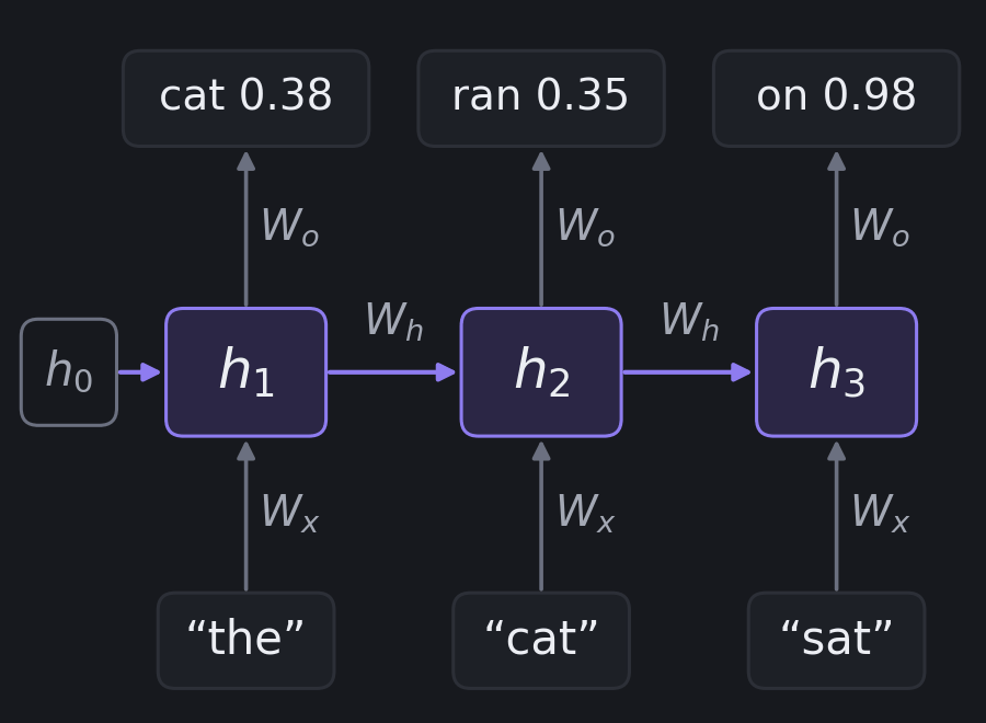
For example, when the RNN reads “the cat sat,” the state after “the” is \(h_1\). When it reads “cat,” it combines the embedding for “cat” with \(h_1\) to make \(h_2\). When it reads “sat,” it combines that word's embedding with \(h_2\) to make \(h_3\).
The hidden state does not store words in labeled slots. It is a learned numerical summary. It may retain information useful for the task and lose other information.
Why are there two weight matrices?
The two inputs come from different spaces and play different roles:
- The word embedding tells the RNN what is arriving now.
- The previous hidden state carries what the RNN has represented from the past.
Each needs its own transformation before the two contributions can be combined.
\(W_x x_t\): what the current word contributes
\(W_x\) transforms the current word's embedding into the hidden-state space. It determines how features of this word contribute to the new state.
Imagine an embedding with 300 numbers and a hidden state with 512 numbers. Then \(W_x\) has 512 rows and 300 columns:
$$ x_t \in \mathbb{R}^{300}, \qquad W_x \in \mathbb{R}^{512\times300}, \qquad W_xx_t \in \mathbb{R}^{512} $$
Each output number is a weighted combination of the 300 embedding numbers. The transformation does not merely append 212 extra numbers. It computes 512 new combinations of the original features.
A row of \(W_x\) can be pictured as asking, “How much does this word point in a direction that matters for this hidden-state coordinate?” Training determines which combinations are useful. A coordinate might respond to a combination of features that helps the model predict what comes next, but the coordinates do not necessarily have simple human-readable labels like “animal.” Those labels are only intuition, not something the model is explicitly given.
Here is a small numerical illustration. Suppose a word has a two-number embedding:
$$ x_t = \begin{bmatrix}0.9\\0.2\end{bmatrix}, \qquad W_x = \begin{bmatrix}1.5&0.5\\0.25&1\end{bmatrix} $$
Then:
$$ W_xx_t = \begin{bmatrix} 1.5(0.9)+0.5(0.2)\\ 0.25(0.9)+1(0.2) \end{bmatrix} = \begin{bmatrix}1.45\\0.425\end{bmatrix} $$
The word's original coordinates were \((0.9, 0.2)\); its contribution in hidden-state coordinates is now \((1.45, 0.425)\). The learned matrix has mixed and scaled the original features. This result is only the word's contribution; it is not yet the new hidden state.
\(W_h h_{t-1}\): what the previous context contributes
\(W_h\) transforms the previous hidden state. Unlike \(W_x\), it does not map from word-embedding space. It maps from hidden-state space back into hidden-state space, so its result can be combined with the current word's contribution.
For example, let the previous state be:
\(h_{t-1}=\begin{bmatrix}0.8\\0.2\end{bmatrix}\)
Then:
$$ W_hh_{t-1}= \begin{bmatrix} 0.5(0.8)-0.3(0.2)\\ 0.4(0.8)+0.6(0.2) \end{bmatrix} = \begin{bmatrix}0.34\\0.44\end{bmatrix} $$
The second output coordinate receives information from both coordinates of the old state. This is a key job of a matrix: it can combine information across dimensions instead of copying each number straight across. Depending on its learned values, \(W_h\) can preserve, reduce, amplify, or redirect parts of the previous state.
This is how earlier words can affect later updates. The model is not handed a rule such as “remember the subject.” During training, prediction errors adjust \(W_h\) so that useful information in previous states can help with future predictions. \(W_h\) itself stays the same while the model reads a sentence; the state it transforms changes at each word.
The two contributions meet
The outputs of the two matrices now have the same size: both are vectors in hidden-state space. The RNN can add them:
$$ W_hh_{t-1} + W_xx_t $$
If the model used only \(W_xx_t\), the new state would not depend on earlier words. Starting from the same state, different histories would have no effect. If it used only \(W_hh_{t-1}\), it could update its existing context but would not bring in the new word. It needs both sources to respond to the current word in light of what came before.
The bias \(b\): a learned nudge
The bias is a learned vector added to the two contributions. It gives each hidden-state coordinate a baseline adjustment, even when the two transformed inputs happen to be zero. A negative bias nudges a coordinate down; a positive bias nudges it up. Training learns these adjustments along with the matrices.
The bias has one number per hidden-state coordinate. If the hidden state has 512 numbers, \(b\) has 512 numbers too.
One complete worked step
Now combine all the pieces in one small example. To keep the arithmetic visible, use two-number vectors throughout. These values are illustrative; they are not claimed to be the learned values for any particular word or model.
Suppose the previous state summarizes the text before the word “cat,” and “cat” has this embedding:
\(h_{t-1}=\begin{bmatrix}0.8\\0.2\end{bmatrix}\), \(x_t=\begin{bmatrix}0.9\\0.2\end{bmatrix}\)
Use the matrices from the examples above, and choose this bias:
\(W_h=\begin{bmatrix}0.5&-0.3\\0.4&0.6\end{bmatrix}\), \(W_x=\begin{bmatrix}1.5&0.5\\0.25&1\end{bmatrix}\), \(b=\begin{bmatrix}-0.2\\0.1\end{bmatrix}\)
1. Transform the previous state.
0.5 × 0.8 − 0.3 × 0.2 = 0.34
0.4 × 0.8 + 0.6 × 0.2 = 0.44
This is the contribution from the context already carried forward.
2. Transform the current word.
1.5 × 0.9 + 0.5 × 0.2 = 1.45
0.25 × 0.9 + 1 × 0.2 = 0.425
This is the contribution from “cat.”
3. Add both contributions and the bias.
0.34 + 1.45 + (−0.2) = 1.59
0.44 + 0.425 + 0.1 = 0.965
The vector \(z\) is the combined, pre-activation result. It is not yet the new hidden state.
4. Apply tanh to each number.
tanh(1.59) ≈ 0.92
tanh(0.965) ≈ 0.75
So the new state is approximately \((0.92, 0.75)\). It reflects both the previous context and the current word, after the learned transformations, bias, and tanh have been applied. The RNN passes this new state forward to process the next word.
Why apply tanh?
Before tanh, the combined vector \(z\) can contain any real numbers, including very large positive or negative values. tanh applies the same nonlinear function to each coordinate and puts each result between −1 and 1:
Before tanh |
After tanh (approximately) |
|---|---|
| −3 | −0.995 |
| −1 | −0.762 |
| 0 | 0 |
| 1 | 0.762 |
| 3 | 0.995 |
This has two useful effects:
- It bounds the state values. Every coordinate of the new state stays between −1 and 1, rather than growing without limit in a single update.
- It adds nonlinearity. The matrix operations and addition alone are linear or affine. Without a nonlinear step, repeatedly updating the state would remain a linear or affine calculation of the inputs.
tanhlets the RNN represent more complex relationships between the current word and the previous context.
Geometrically, \(W_x\) and \(W_h\) first move and reshape their contributions in hidden-state space. Addition combines them into \(z\). Then tanh bends and compresses each coordinate to produce a point inside the bounded hidden-state region.
A limitation: bounding the state does not guarantee that the RNN preserves useful information. For very large inputs, tanh outputs get close to −1 or 1, so different large values become hard to distinguish. Its slope also becomes small there, which can make learning long-range dependencies difficult. This contributes to the vanishing-gradient problem discussed in treatments of RNN training.
How the state carries a sequence
The equation is applied repeatedly:
$$ \begin{aligned} h_1 &= \tanh(W_hh_0 + W_xx_1+b) \\ h_2 &= \tanh(W_hh_1 + W_xx_2+b) \\ h_3 &= \tanh(W_hh_2 + W_xx_3+b) \end{aligned} $$
Often the initial state \(h_0\) is set to zero. After the first word, each state depends on the state before it. That means \(h_3\) can be influenced by words 1, 2, and 3, even though the immediate input at step 3 is only \(x_3\).
The weights \(W_x\), \(W_h\), and \(b\) are shared across all these steps. The inputs and hidden states change; the learned update rule does not. This lets the same RNN process sequences of different lengths without making a new set of weights for every word position. In practice, information from far back may fade, so “can be influenced by” does not mean “remembers everything perfectly.”
Where do the weights come from?
The matrices and bias are learned from examples. For a next-word prediction task, the RNN uses its state to produce scores for possible next words. A separate output layer might compute:
$$ \text{scores}=W_o h_t+c, \qquad p(\text{next word})=\text{softmax}(\text{scores}) $$
The scores become probabilities, and the training process compares those probabilities with the actual next word. It adjusts the embeddings, matrices, biases, and output layer to make future predictions better. Through this process, \(W_x\) learns how words should contribute, \(W_h\) learns how previous states should contribute, and \(b\) learns its coordinate-wise nudges. They are optimized together for the task; they are not separately assigned hand-written meanings like “animal detector” or “subject memory.”
In one sentence: the RNN transforms what it sees now and what it has carried from before, combines them, and turns that combination into the next version of its summary.
The calculation above used small illustrative values to make each part of the update easy to see. Now let's run one step using the actual learned values from our tiny model.
One step using the trained model
Let's run one step by hand. Throughout this tutorial we'll use a deliberately tiny model so that every number is visible. It's trained on 16 sentences built from this pattern:
the {cat, dog, bird} {sat on, slept on, ran to} the {mat, rug} or {door, park} .
Sat and slept are followed by on, then mat or rug; ran is followed by to, then door or park. During training the sentences are shuffled and glued end to end into one long stream of text, so the model also has to cope with whatever came before each sentence. One combination is held out on purpose: the training data never contains "the bird sat". We'll use that later to test generalization. The vocabulary has 14 tokens (counting the period), each word embedding has 2 numbers, and the hidden state has 2 numbers, so we can plot both directly. The training code is at the end; every number below comes from it.
After reading "the", the model's hidden state is \(h_1 = (-0.97,\ -0.99)\). Now it reads "cat", whose learned embedding is \(x_2 = (-0.95,\ -0.48)\). The trained weights, rounded to two decimals, are:
$$W_h = \begin{bmatrix} 3.10 & 0.38 \\ -0.32 & -0.05 \end{bmatrix}, \quad W_x = \begin{bmatrix} 1.94 & 1.48 \\ 1.53 & -1.30 \end{bmatrix}, \quad b = \begin{bmatrix} 0.25 \\ 0.45 \end{bmatrix}$$
The memory term carries the old state forward:
$$W_h h_1 = \begin{bmatrix} 3.10(-0.97) + 0.38(-0.99) \\ -0.32(-0.97) - 0.05(-0.99) \end{bmatrix} = \begin{bmatrix} -3.38 \\ 0.36 \end{bmatrix}$$
The input term brings in the new word:
$$W_x x_2 = \begin{bmatrix} 1.94(-0.95) + 1.48(-0.48) \\ 1.53(-0.95) - 1.30(-0.48) \end{bmatrix} = \begin{bmatrix} -2.55 \\ -0.83 \end{bmatrix}$$
Add them with the bias, then squash:
$$h_2 = \tanh\left(\begin{bmatrix} -3.38 - 2.55 + 0.25 \\ 0.36 - 0.83 + 0.45 \end{bmatrix}\right) = \tanh\left(\begin{bmatrix} -5.68 \\ -0.02 \end{bmatrix}\right) = \begin{bmatrix} -1.00 \\ -0.02 \end{bmatrix}$$
With full-precision weights the model gets \((-1.00,\ 0.00)\); the small gap in the second number is rounding.
The two numbers tell two different stories. In the first, the memory term (−3.38) and the word "cat" (−2.55) push the same way, and the sum of −5.68 is so large that tanh pins it at −1. In the second, memory pushes up, the word pushes down, and the bias nearly cancels what's left, so the result lands at zero. The new state is a negotiation between where you were and what you just read. From \(h_2\) the model predicts ran 0.35, slept 0.35, sat 0.29: after "the cat", a verb comes next.
Memory as a Moving Point
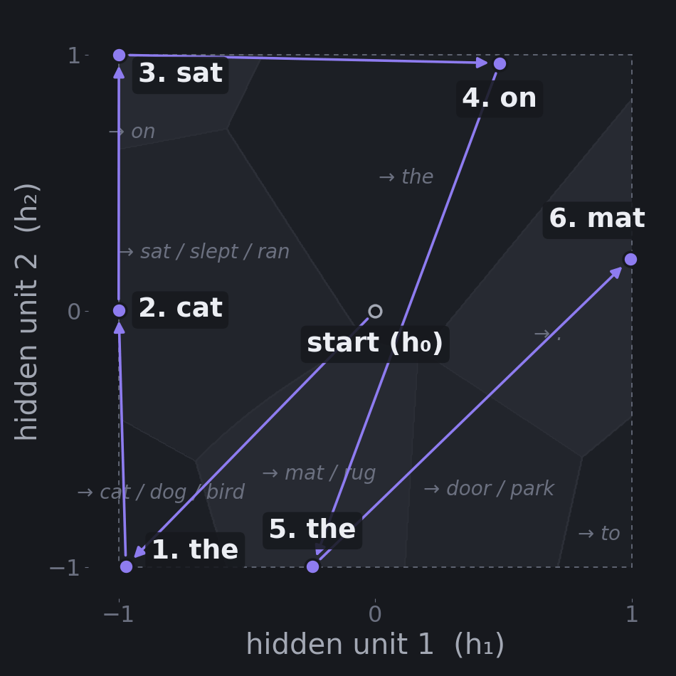
Here's the central picture. The hidden state is one point. Our model's hidden state has two numbers, so the point lives on a flat square from −1 to 1 in each direction (tanh can't go further). The point starts at the origin. Each word moves it somewhere new. Wherever it lands decides what the model predicts next.
Follow the point:
Each dot is the hidden-state vector, shown as a pair of numbers. The first number sets its left-to-right position on the horizontal axis; the second sets its up-and-down position on the vertical axis. For each word, it calculates \(h_t=\tanh(W_h\,h_{t-1}+W_x\,x_t+b)\): it combines the previous state and the new word’s embedding using learned weights, adds a bias, then applies tanh to each result. The two resulting numbers give the point’s coordinates. The weights and word embeddings were learned during training; the plotted coordinates are the model’s calculated hidden states, rounded to two decimal places. For example, after the first word, “the,” the hidden-state vector is about [−0.97, −0.99], so its dot is near the square’s lower-left corner.
Because tanh maps each number to a value between −1 and 1, every point stays inside this square. Values shown as exactly −1.00 or 1.00 are rounded: for finite inputs, tanh gets close to those limits but does not reach them. The gray regions group locations by which next word scores highest. We grouped words for display; the trained model’s output layer determines the boundaries.
| After reading | Hidden state \(h\) | Model's top predictions |
|---|---|---|
| the | (−0.97, −0.99) | cat 0.38, dog 0.37, bird 0.24 |
| the cat | (−1.00, 0.00) | ran 0.35, slept 0.35, sat 0.29 |
| the cat sat | (−1.00, 1.00) | on 0.98 |
| the cat sat on | (0.49, 0.97) | the 1.00 |
| the cat sat on the | (−0.24, −1.00) | rug 0.48, mat 0.48 |
| the cat sat on the mat | (0.99, 0.20) | . 0.99 |
What determines the predictions?
The hidden-state vector is the summary the RNN has made so far. A separate output layer uses that summary to score each possible next word.
It gives each of the toy model’s 14 possible outputs—including the period—a score. You can think of a score as how strongly the current summary points toward that word. The output layer uses learned weights \(W_o\) and a learned bias \(c\):
\(\text{scores}\) = \(W_o\) × \(h_t\) + \(c\)
This tiny model has a two-number hidden state and 14 possible next words. So \(W_o\) has 14 rows and 2 columns: one two-number scoring row for each possible word. The matching entry in \(c\) is that word’s bias. Multiplying a row by the hidden-state vector and adding its bias gives that word one score. The model repeats this for all 14 rows, producing 14 scores.
For example, suppose the hidden state is \([0.2, 0.8]\). To score on, imagine its learned row were \([1.0, 0.5]\) and its bias were −0.1. Then its score would be:
1.0 × 0.2 + 0.5 × 0.8 − 0.1 = 0.5
Those numbers are just to demonstrate the calculation; training learns the actual weights and biases. The row for on is a scoring rule, not an embedding or a point to measure distance from. The score comes from multiplying and adding coordinates, not from geometric closeness.
These raw scores help rank the choices, but they are not probabilities. They can be negative or positive, and they do not add up to 1. So a raw score by itself does not tell us “the model gives this word a 98% chance.”
Softmax turns those scores into probabilities. It converts all the scores together into probabilities between 0 and 1 that add up to 1—a 100% share across the possible next words. A word with a much higher score gets most of that share; words with similar scores split it.
For example, after “the cat sat,” on gets a 0.98 probability, so the model assigns nearly all its share to on. After “the cat sat on the,” mat and rug get about 0.48 each, so the model is nearly split between them. The table shows only the top predictions, rounded to two decimal places; the rest of the probability is assigned to other words.
Each step does two jobs at once. It remembers: the new hidden-state vector depends on the previous one. It also positions for prediction: the new position receives scores from the output layer.
Locations where the same word gets the highest score form that word’s prediction region. These regions are a picture of which score wins; they are not based on distance to a word embedding. During training, the model learns both how words move the hidden-state point and how the output layer scores each location.
Three things in this picture are worth noticing:
- The predictions are honest about uncertainty. After "the cat sat on the", the model splits evenly between mat and rug, because in the training data both are equally common. A good language model shouldn't be certain when the data isn't.
- Many points sit on the edges of the square. Making confident predictions from only two numbers means pushing the state to extremes, so the model leans on tanh's limits of −1 and 1. Small models often do this, and it has a cost we'll meet in the section on vanishing gradients.
- The axes don't have meanings. It's tempting to read the horizontal axis as "noun-ness" or similar. Don't. Training could just as well have swapped or flipped the axes, and in real models with hundreds of dimensions, information is spread across combinations of units rather than assigned one feature per unit. What matters is where points land relative to each other and to the prediction regions.
Hidden states can still capture patterns that help with prediction. For example, if contexts involving cats, dogs, and birds tend to lead to similar next words in the training data, the model may place some of those states near one another. That similarity emerges from learning to predict; no coordinate or region is pre-labeled “animal.” What the state captures depends on the task and training examples.
Real RNNs have hidden states with hundreds of dimensions, so you can't plot them directly. The picture is the same, though: one point, moving one word at a time, in a space carved into regions that predict different next words.
The same word lands in different places
If the hidden state were just a function of the current word, "the" would always land in the same place. It doesn't.
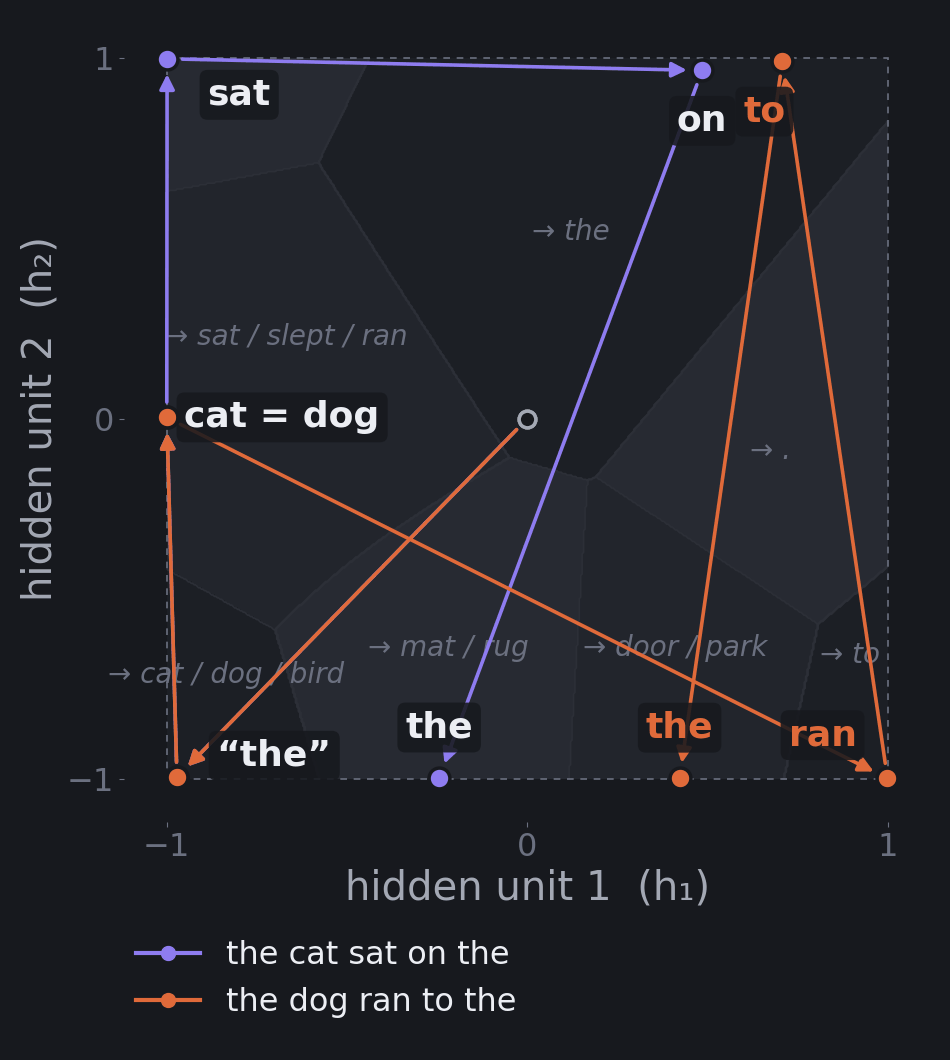
| Context | Where "the" lands | Top predictions |
|---|---|---|
| start of text | (−0.97, −0.99) | cat 0.38, dog 0.37, bird 0.24 |
| the cat sat on the | (−0.24, −1.00) | rug 0.48, mat 0.48 |
| the dog ran to the | (0.42, −1.00) | door 0.46, park 0.46 |
| the cat sat on the mat . the | (−0.95, −1.00) | cat 0.37, dog 0.37, bird 0.24 |
The middle pair is the interesting one. To know whether a mat/rug or a door/park comes next, the model has to remember whether it saw on or to two words ago. That memory is stored entirely in where the point sits.
The last row shows the opposite skill. After a period, "the" lands at essentially the same point as at the very start of the text, whatever the previous sentence was about (after "the dog ran to the park ." it lands in the same spot). Because the model was trained on sentences glued together, it learned to treat the period as a reset: the old sentence no longer helps predict the new one, so it's wiped out. Remembering and forgetting are both learned. Also notice that "the cat" and "the dog" land on essentially the same point; we'll see why in the next section.
You can drive the model yourself. The explorer below runs the actual trained weights in your browser. Pick a sentence or add words one at a time and watch the point move and the predictions change.
Explore the trained RNN
What Each Word Owns, and What Everyone Shares
An RNN has two kinds of parameters, and the difference explains a lot about why it works.
Each word owns its embedding. The embedding table has one row per word in the vocabulary. When the model reads "cat", it looks up the cat row, and only that row. Here are some of our model's learned embeddings:
| Word | Learned embedding |
|---|---|
| cat | (−0.95, −0.48) |
| dog | (−0.92, −0.46) |
| bird | (−0.72, −0.49) |
| mat | (0.92, 1.37) |
| rug | (0.93, 1.38) |
| door | (0.48, 0.70) |
| park | (0.53, 0.75) |
| sat | (0.60, −1.44) |
| slept | (0.56, −2.42) |
Cat and dog ended up 0.03 apart, and bird sits close by. Mat and rug are nearly identical, and door and park are close too. Nobody told the model that these words are similar. They appear in the same company in the training data, so training gave them similar vectors. That's exactly the word2vec idea from The Company Words Keep, arising here as a side effect of predicting the next word. It's also why "the cat" and "the dog" land on essentially the same point.
Sat and slept are less alike: they're almost a full unit apart (0.98). Both are followed by "on", but they don't keep quite the same company, because no bird ever sat in the training data. The likely reason for the gap is that the two words aren't interchangeable in this corpus, so training had no pressure to merge them.
Everyone shares the rest. \(W_x\), \(W_h\), \(b\), \(W_o\), and \(c\) are used for every word, at every position, in every sentence. Think of the embeddings as each word's identity, and the shared weights as one set of rules for how any word changes the context and what the context predicts.
Sharing buys three things:
- Any length works. The same rules apply at step 3 and at step 300.
- Lessons transfer. What the model learns about "sat" at position 3 applies wherever "sat" appears, and what it learns about moving from a noun to a verb applies to every noun.
- Size doesn't grow with the sentence. Parameters depend on vocabulary size and layer widths, never on how much text you feed in.
Counting the parameters
Let's count for a realistic model: a 10,000-word vocabulary, 300-dimensional embeddings, and a 512-dimensional hidden state.
| Piece | Shape | Parameters |
|---|---|---|
| Word embeddings | 10,000 × 300 | 3,000,000 |
| \(W_x\) (input to hidden) | 512 × 300 | 153,600 |
| \(W_h\) (hidden to hidden) | 512 × 512 | 262,144 |
| \(b\) (hidden bias) | 512 | 512 |
| \(W_o\) (hidden to output) | 10,000 × 512 | 5,120,000 |
| \(c\) (output bias) | 10,000 | 10,000 |
| Total | 8,546,256 |
About 8.55 million parameters. Two things stand out:
- 95% of them live in the two vocabulary-sized tables, the embeddings and \(W_o\). The recurrent core that does the "remembering" (\(W_x\), \(W_h\), and \(b\)) is only 416,256 parameters, under 5% of the total.
- The recurrent step costs about the square of the hidden size. Updating a 512-number hidden state takes about 512 × 512 ≈ 262,000 multiply-adds in \(W_h\) alone, for every token. Double the hidden size and that cost quadruples. Worse, the steps have to run one after another: you can't compute the state at word 50 until you have the state at word 49, so a long text can't be split across positions and processed in parallel. That combination is one reason hidden states can't simply be made enormous.
Our toy model has \(14 \times 2 = 28\) embedding weights, \(2 \times 2 + 2 \times 2 + 2 = 10\) in the recurrent core, and \(14 \times 2 + 14 = 42\) in the output layer: 80 parameters, which matches what the code prints.
Three Spaces and the Bridges Between Them
Those 8.5 million weights don't create one giant space. An RNN works with three separate spaces, and the weight matrices are the bridges between them:
- Embedding space (300 dimensions in the big example, 2 in ours). Each word is a fixed point here.
- Hidden space (512 dimensions, or 2 in ours). This is where the moving point lives.
- Output space (one dimension per vocabulary word: 10,000, or 14 in ours). Each point here is a set of scores, one per word.
\(W_x\) is the bridge from embedding space into hidden space. \(W_h\) is a bridge from hidden space back into itself, which is what makes the network recurrent. \(W_o\) is the bridge from hidden space out to the vocabulary.
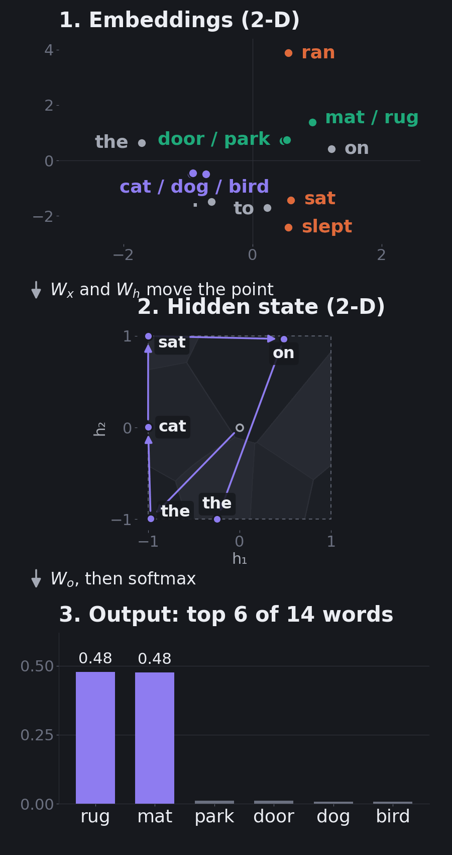
A common worry: going from 512 numbers to 10,000 sounds like spreading information thin, as if most of the 10,000 outputs must be empty. It isn't. Each word \(w\) gets its own row \(u_w\) of \(W_o\), a direction in hidden space, and its score is
$$z_w = u_w \cdot h + c_w$$
So all 10,000 scores are computed from the same 512 numbers, each one asking "how far does the hidden state point in my direction?" Nothing is sparse. The scores just aren't independent: they're 10,000 different readings of one 512-dimensional point. Going from 300 to 512 works the same way in the other direction: every hidden unit is a weighted combination of all 300 embedding numbers, a new "view" of the word rather than the same numbers padded with zeros.
From a point to a probability
Let's turn a real hidden state into a prediction. After reading "the", the state is \(h = (-0.972,\ -0.995)\) (three decimals this time, because the scores below are large enough that rounding matters). The row of \(W_o\) for cat is \((-13.50,\ -10.03)\) and its bias is −9.49, so its score (called a logit) is
$$z_{\text{cat}} = -13.50(-0.972) - 10.03(-0.995) - 9.49 = 13.61$$
Doing the same for every word gives dog 13.59, bird 13.16, sat 9.36, rug 9.18, and lower scores for everything else. Scores can be any size, so softmax turns them into probabilities that are positive and sum to 1:
$$p_i = \frac{e^{z_i}}{\sum_j e^{z_j}}$$
Subtracting the largest score from every score doesn't change the result and keeps the numbers small. Relative to cat: \(e^{0} = 1\), \(e^{-0.02} = 0.98\) for dog, \(e^{-0.45} = 0.64\) for bird, and the other eleven words add up to only 0.04. The total is 2.66, so
$$p_{\text{cat}} = \frac{1}{2.66} = 0.38, \qquad p_{\text{dog}} = \frac{0.98}{2.66} = 0.37, \qquad p_{\text{bird}} = \frac{0.64}{2.66} = 0.24$$
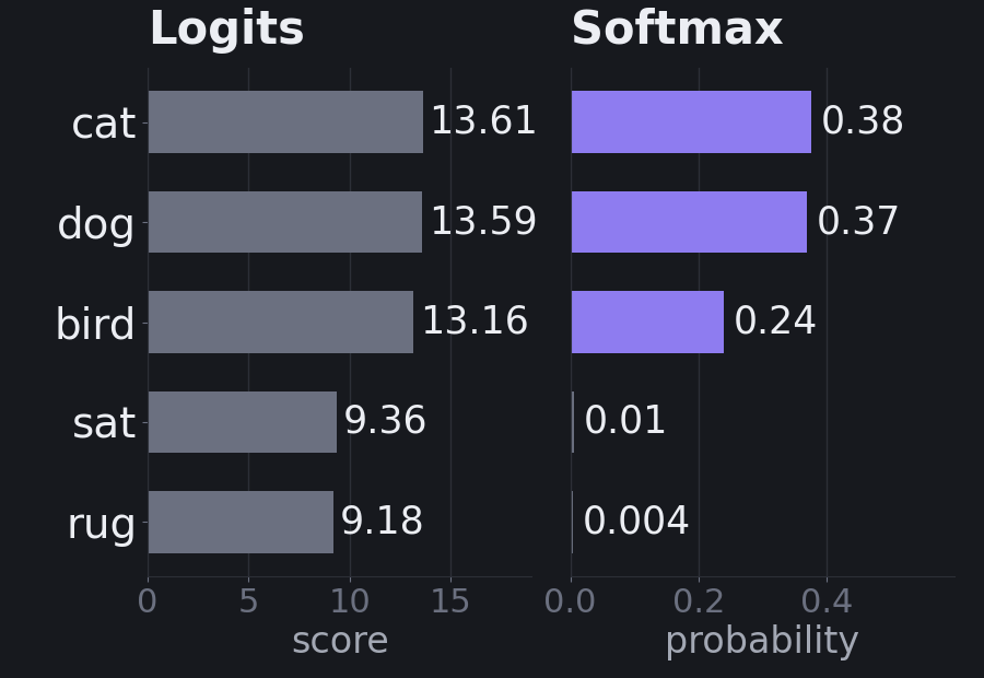
A check: in the training data, sentences start with "the cat" 6 times out of 16, "the dog" 6 times, and "the bird" 4 times: 0.375, 0.375, and 0.25. The model learned almost exactly those odds.
Why these two functions? tanh for the hidden state because the state is fed back into itself at every step. Bounding it between −1 and 1 keeps it from growing without limit over a long sentence, and being centered on zero lets each unit push in either direction. Softmax for the output because we need a probability distribution over the vocabulary to compare against the word that actually came next.
Training: Learning From Next-Word Prediction
Where do the weights come from? From a game the model plays with itself: read some text, guess the next word, check, adjust.
Every position in the text is a training example. "the cat sat on the mat ." gives six of them: the → cat, the cat → sat, the cat sat → on, and so on, and in a stream of sentences the period gives one more, . → the. Each training step shuffles the 16 sentences into 8 different streams of 112 tokens and asks for every next word: 8 × 111 = 888 predictions per step.
The loss is cross-entropy: the negative log of the probability the model gave to the word that actually came next.
$$L = -\log p(\text{correct word})$$
If the model gave the right word 0.99, the loss is 0.01. If it gave 0.37, the loss is 0.99. If it gave 0.01, the loss is 4.61. Confident and wrong is punished hard. Training minimizes the average over all 888 predictions.
Our model starts at a loss of 2.635, about what you'd get from guessing uniformly among 14 words (\(\ln 14 = 2.64\)). After 1,500 steps it reaches 0.423. It can't reach zero, because the data itself is uncertain: after "the", any of three animals can follow. A model that knew the exact odds inside each sentence would score about 0.40, so the tiny model is close to that.
Backpropagation through time
To improve the weights we need gradients, and the unrolled picture tells us how to get them. The loss at step 4 depends on \(h_4\). But \(h_4\) was computed from \(h_3\), which came from \(h_2\), and so on back to the first word. So the gradient flows backward through every earlier step. This is called backpropagation through time (BPTT). It's ordinary backpropagation applied to the unrolled network.
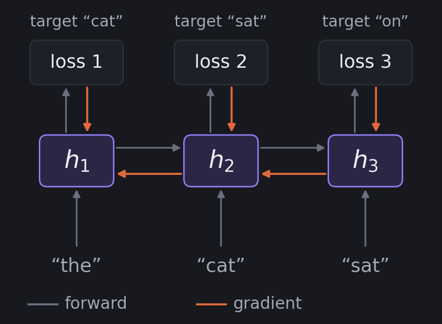
Because the weights are shared, every step contributes to the gradient of the same \(W_h\), \(W_x\), and \(W_o\), and those contributions are added together. Then one gradient-descent step nudges each weight downhill, exactly as in Introduction to Machine Learning. In PyTorch, all of this happens inside one call to loss.backward().
Generalization by Proximity
Remember the held-out sentence. The model never saw "the bird sat". What does it do with it?
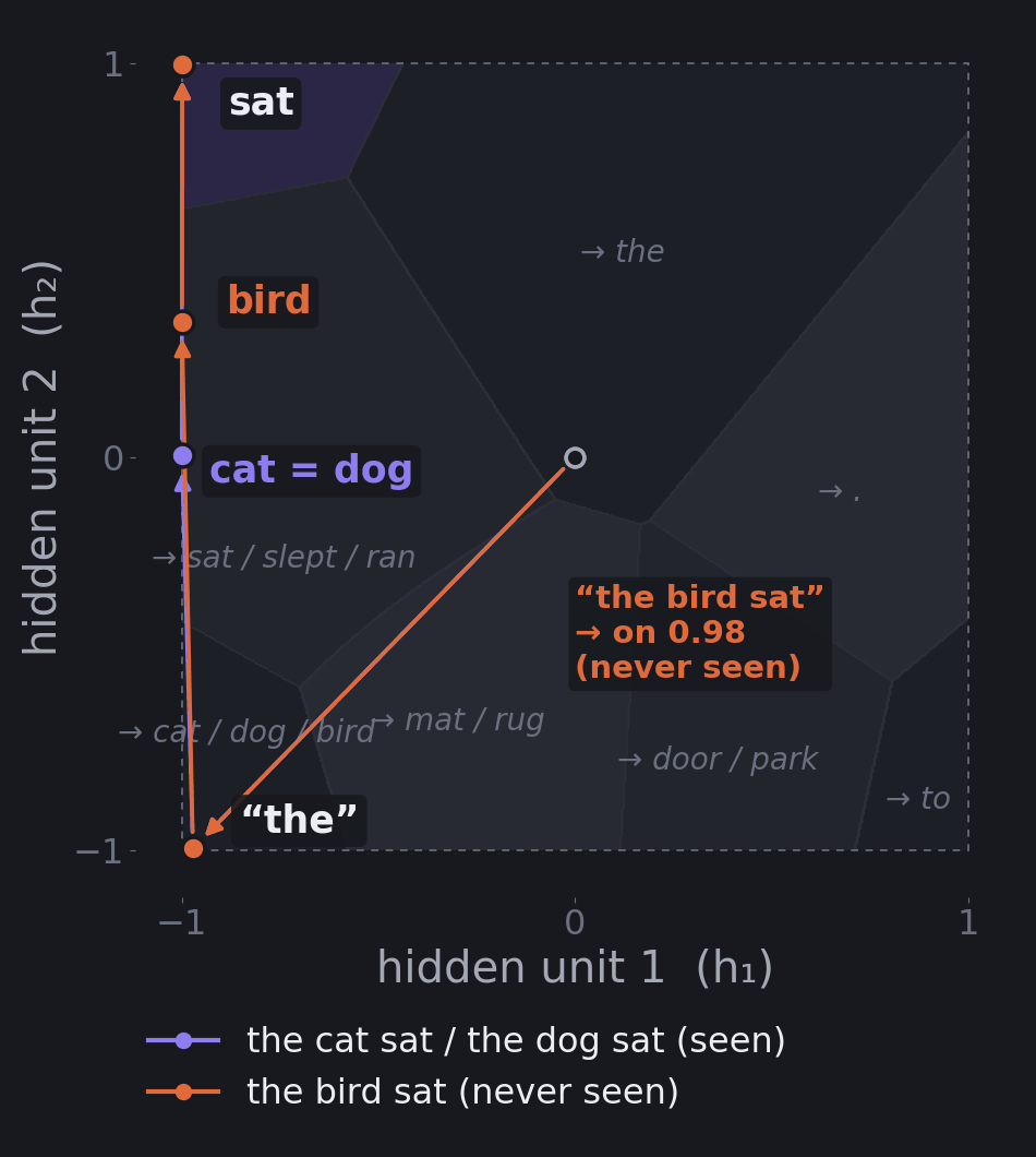
| Prefix | Hidden state | Top predictions |
|---|---|---|
| the cat | (−1.00, 0.00) | ran 0.35, slept 0.35, sat 0.29 |
| the bird | (−1.00, 0.34) | slept 0.44, ran 0.43, sat 0.09 |
| the cat sat | (−1.00, 1.00) | on 0.98 |
| the dog sat | (−1.00, 1.00) | on 0.98 |
| the bird sat | (−1.00, 1.00) | on 0.98 |
Two things happened, and both are reasonable.
First, the model noticed the gap. It gives sat only 0.09 after "the bird", versus 0.29 after "the cat". In its training data, birds never sat.
Second, when it does see "the bird sat", it reuses what it knows. Bird shares company with cat and dog (they all slept and ran in the same places), so its embedding is close to theirs: 0.22 away from cat, compared with 2.63 between cat and mat. A nearby embedding produces a nearby hidden state: "the bird" lands 0.34 from "the cat", and the shared update for sat carries both to the same corner of the square. "the bird sat" ends up at the same point as "the cat sat", inside the region that predicts on, and the model predicts on with probability 0.98.
This is how RNNs, and neural language models in general, handle combinations they've never seen. Similar contexts land in similar places, and nearby places make similar predictions. It cuts both ways, though. Proximity transfers patterns whether or not they're true, so a model can transfer a pattern that happens not to hold.
Where Simple RNNs Struggle
Vanishing and exploding gradients
Backpropagation through time multiplies. To see how much the final state depends on a state \(k\) steps earlier, you chain one factor per step:
$$\frac{\partial h_T}{\partial h_{T-k}} = \frac{\partial h_T}{\partial h_{T-1}} \cdot \frac{\partial h_{T-1}}{\partial h_{T-2}} \cdots \frac{\partial h_{T-k+1}}{\partial h_{T-k}}$$
and each factor is the same kind of thing:
$$\frac{\partial h_t}{\partial h_{t-1}} = \text{diag}\left(1 - h_t^2\right) W_h$$
The first part is the slope of tanh at each unit. It's at most 1, and it's close to 0 when a unit is saturated near −1 or 1. The second part is the recurrent matrix, the same one at every step. Multiply many of these together and the result behaves like a number raised to a power: if the factors are typically smaller than 1, the product shrinks exponentially; if they're typically larger, it grows exponentially.
Let's measure it on our trained model. The snippet below picks up where the full program at the end of this tutorial leaves off (it uses the trained model and the stoi lookup from there). It feeds in a 28-word stream of four sentences back to back, the same kind of continuous text the model was trained on, and walks backward from the last word, printing each step's factor and the running product.
# Run after tiny_rnn.py (full listing at the end of this tutorial).
# How much does the last hidden state still depend on the state k steps
# earlier? Each step back multiplies by that step's Jacobian
#   dh_t/dh_{t-1} = diag(1 - h_t^2) @ W_h
stream = ("the cat sat on the mat . the dog ran to the park . "
          "the bird slept on the rug . the cat ran to the door .").split()
with torch.no_grad():
    _, states = model(torch.tensor([[stoi[w] for w in stream]]))
h = states[0]                                  # (28, 2): one point per word
W_h = model.W_h.weight.detach()
norm = lambda M: torch.linalg.matrix_norm(M, ord=2).item()

print(f"largest stretch W_h can apply: {norm(W_h):.2f}\n")
print(" k  word read  h after it       tanh slopes     step  total")
J = torch.eye(2)
for k in range(1, 9):
    h_t = h[-k]
    slope = 1 - h_t ** 2                       # tanh'(.) at each unit
    step = torch.diag(slope) @ W_h
    J = J @ step
    print(f"{k:2d}  {stream[-k]:<9} ({h_t[0]:+.2f}, {h_t[1]:+.2f})  "
f"({slope[0]:.3f}, {slope[1]:.3f}) {norm(step):5.3f} {norm(J):.1e}")largest stretch W_h can apply: 3.14
k word read h after it tanh slopes step total
1 . (-0.01, +0.79) (1.000, 0.374) 3.128 3.1e+00
2 door (+1.00, +0.18) (0.007, 0.966) 0.314 4.7e-02
3 the (+0.42, -1.00) (0.821, 0.006) 2.568 1.2e-01
4 to (+0.71, +0.99) (0.499, 0.016) 1.560 1.8e-01
5 ran (+1.00, -1.00) (0.001, 0.004) 0.005 7.9e-04
6 cat (-1.00, -0.00) (0.000, 1.000) 0.324 3.1e-05
7 the (-0.95, -1.00) (0.096, 0.009) 0.299 9.0e-06
8 . (-0.01, +0.79) (1.000, 0.375) 3.128 2.8e-05\(W_h\) on its own could stretch a vector by up to 3.14, so you might expect explosion. The "step" column shows what actually happens. Our model's memory runs mostly through the first hidden unit: its row of \(W_h\) is \((3.10,\ 0.38)\), while the second unit's row is a weak \((-0.32,\ -0.05)\). Whenever the first unit is pinned near ±1, as after door and cat, its tanh slope is close to 0, that strong path is cut, and only the weak one is left, so the step shrinks to about 0.3. After ran, both units are pinned and the step is 0.005: almost nothing gets through. Three of the eight steps stretch by more than 2.5, yet eight steps back the total is down to 0.000028. It can fall even faster than the step sizes multiply, because each step stretches in a different direction and a stretch in one direction doesn't help a signal pointing another way. Saturation doesn't concentrate the gradient on a few important words; it cuts the path, and whatever lies behind a cut gets almost no signal.
The same measurement on a 64-unit version of the model, trained the same way on the same streams, shows the more typical pattern:
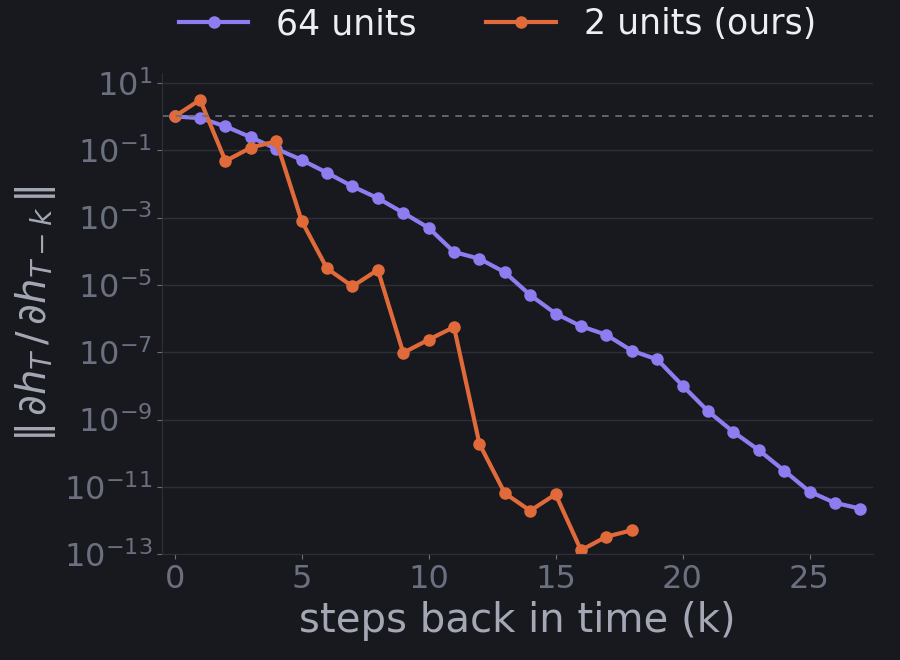
The bigger model's signal shrinks smoothly, roughly halving with each step back, and falls below \(10^{-4}\) by 11 steps back. That's the vanishing gradient problem: the training signal from a prediction can't reach words far in the past, so the model has trouble learning that they matter. Consider "The keys that I left on the kitchen table yesterday ___". Choosing are over is depends on keys, eight words back. If the gradient shrinks like this, the signal reaching keys is tiny, so the model learns that connection slowly, if at all.
The opposite failure, exploding gradients, happens when the factors are mostly larger than 1. Gradients become huge, a single update throws the weights far off, and the loss jumps or turns into NaN. The standard fix is gradient clipping: if the gradient's overall length exceeds a threshold, scale it down to that length before the update. Our training loop does this with clip_grad_norm_(model.parameters(), 1.0). Clipping tames explosions, but it does nothing for vanishing gradients; you can't rescale a signal that's already gone.
Everything squeezed into one point
There's a second, simpler limit. The hidden state is a fixed-size vector, and it's overwritten at every step. Everything the model knows about the past has to fit in that one point, and each new word partly erases what was there. A basic RNN also has no way to look back at a specific earlier word and decide it matters more than the others. Whatever survived in the hidden state is all it has.
What Came Next
Each of the main successors to the basic RNN attacks one of these limits.
LSTM (long short-term memory; Hochreiter and Schmidhuber, 1997; the forget gate was added by Gers et al. in 2000) adds a second vector, the cell state, plus three gates: small sigmoid layers that output values between 0 and 1 and decide what to forget, what to write, and what to reveal. The cell state is updated mostly by adding and scaling rather than by squashing through tanh with a full matrix multiply at every step. When the forget gate stays near 1, the gradient can travel back along the cell state for many steps without vanishing.
GRU (gated recurrent unit, Cho et al., 2014) simplifies the LSTM to two gates and a single state vector. It often performs about as well with fewer parameters.
Attention (Bahdanau, Cho, and Bengio, 2014) removes the one-point bottleneck. It was introduced for translation: instead of squeezing the whole source sentence into one final hidden state, the decoder keeps all of the encoder's hidden states and, for each word it writes, computes learned weights over them: an explicit answer to "which source words matter right now?" This is the importance mechanism a basic RNN lacks. Transformers (Vaswani et al., 2017) went further, dropping recurrence entirely and building everything from attention. Without the step-by-step chain, they can process every position of a training text in parallel, though generating text still happens one token at a time.
The moving-point picture still applies to LSTMs and GRUs. Their state is still a point moving through space one word at a time; the gates just give the network much finer control over how far, and in which directions, each word is allowed to move it.
The Full Implementation
Here's the complete program behind every number and figure in this tutorial. It writes the RNN loop out by hand so you can see the equation in the code. PyTorch's built-in nn.RNN runs the same loop in optimized form; it keeps two bias vectors (bias_ih_l0 and bias_hh_l0) that simply add together into our single \(b\).
import torch
import torch.nn as nn
import torch.nn.functional as F

torch.manual_seed(12)

# ---------------------------------------------------------------
# 1. A toy corpus: every "the    the  ."
#    except that "the bird sat ..." never appears. We hold it out
#    to test generalization later.
# ---------------------------------------------------------------
subjects = ["cat", "dog", "bird"]
verbs = {"sat": "on", "slept": "on", "ran": "to"}       # verb -> preposition
places = {"on": ["mat", "rug"], "to": ["door", "park"]}  # preposition -> places

sentences = [
    f"the {s} {v} {p} the {o} ."
    for s in subjects
    for v, p in verbs.items()
    for o in places[p]
    if (s, v) != ("bird", "sat")
]
vocab = sorted({w for s in sentences for w in s.split()})
stoi = {w: i for i, w in enumerate(vocab)}
data = torch.tensor([[stoi[w] for w in s.split()] for s in sentences])

print(f"{len(sentences)} sentences, vocabulary of {len(vocab)}: {vocab}")


# ---------------------------------------------------------------
# 2. The model: h_t = tanh(W_h h_{t-1} + W_x x_t + b),  logits = W_o h_t + c
# ---------------------------------------------------------------
class TinyRNN(nn.Module):
    def __init__(self, vocab_size, emb_dim=2, hidden_dim=2):
        super().__init__()
        self.hidden_dim = hidden_dim
        self.embed = nn.Embedding(vocab_size, emb_dim)            # one vector per word
        self.W_x = nn.Linear(emb_dim, hidden_dim)                 # shared; its bias is b
        self.W_h = nn.Linear(hidden_dim, hidden_dim, bias=False)  # shared
        self.W_o = nn.Linear(hidden_dim, vocab_size)              # shared; its bias is c

    def forward(self, tokens):
        batch, steps = tokens.shape
        h = torch.zeros(batch, self.hidden_dim)  # h_0: start at the origin
        states = []
        for t in range(steps):                   # same weights at every step
            x_t = self.embed(tokens[:, t])
            h = torch.tanh(self.W_h(h) + self.W_x(x_t))
            states.append(h)
        states = torch.stack(states, dim=1)      # (batch, steps, hidden_dim)
        return self.W_o(states), states          # logits for every step, plus the path


model = TinyRNN(len(vocab))
n_params = sum(p.numel() for p in model.parameters())
print(f"parameters: {n_params}")

# ---------------------------------------------------------------
# 3. Train on continuous text, the way language models are trained:
#    shuffle the sentences, glue them into one long stream, and let the
#    hidden state flow across sentence boundaries. Loss is next-word
#    cross-entropy at every position; backprop runs through the whole stream.
# ---------------------------------------------------------------
def make_streams(n=8):
    return torch.stack([data[torch.randperm(len(data))].reshape(-1) for _ in range(n)])


optimizer = torch.optim.AdamW(model.parameters(), lr=0.05, weight_decay=0.01)

for epoch in range(1, 1501):
    streams = make_streams()                    # (8, 112): 16 sentences each
    logits, _ = model(streams[:, :-1])          # predict word t+1 from words 1..t
    loss = F.cross_entropy(logits.reshape(-1, len(vocab)), streams[:, 1:].reshape(-1))
    optimizer.zero_grad()
    loss.backward()                                            # BPTT happens here
    torch.nn.utils.clip_grad_norm_(model.parameters(), 1.0)    # gradient clipping
    optimizer.step()
    if epoch in (1, 100, 500, 1500):
        print(f"epoch {epoch:4d}  loss {loss.item():.3f}")


# ---------------------------------------------------------------
# 4. Look inside: where does each prefix land, and what comes next?
# ---------------------------------------------------------------
@torch.no_grad()
def predict(prompt, k=3):
    tokens = torch.tensor([[stoi[w] for w in prompt.split()]])
    logits, states = model(tokens)
    probs = logits[0, -1].softmax(-1)
    top = probs.topk(k)
    h = states[0, -1].tolist()
    guesses = "  ".join(f"{vocab[i]} {p:.2f}" for p, i in zip(top.values.tolist(), top.indices.tolist()))
    print(f"{prompt:<29} h = ({h[0]:+.2f}, {h[1]:+.2f})   next: {guesses}")


print()
for prompt in ["the", "the cat", "the cat sat", "the cat sat on", "the cat sat on the",
               "the dog ran to the", "the cat sat on the mat"]:
    predict(prompt)

print("\nThe same word after different histories:")
for prompt in ["the", "the cat sat on the mat . the", "the dog ran to the park . the"]:
    predict(prompt)

print("\nGeneralization (the model never saw 'the bird sat'):")
for prompt in ["the cat", "the bird", "the cat sat", "the dog sat", "the bird sat"]:
    predict(prompt)
Running it prints:
16 sentences, vocabulary of 14: ['.', 'bird', 'cat', 'dog', 'door', 'mat', 'on', 'park', 'ran', 'rug', 'sat', 'slept', 'the', 'to']
parameters: 80
epoch    1  loss 2.635
epoch  100  loss 0.981
epoch  500  loss 0.470
epoch 1500  loss 0.423

the                           h = (-0.97, -0.99)   next: cat 0.38  dog 0.37  bird 0.24
the cat                       h = (-1.00, +0.00)   next: ran 0.35  slept 0.35  sat 0.29
the cat sat                   h = (-1.00, +1.00)   next: on 0.98  slept 0.01  ran 0.01
the cat sat on                h = (+0.49, +0.97)   next: the 1.00  . 0.00  on 0.00
the cat sat on the            h = (-0.24, -1.00)   next: rug 0.48  mat 0.48  park 0.01
the dog ran to the            h = (+0.42, -1.00)   next: door 0.46  park 0.46  to 0.03
the cat sat on the mat        h = (+0.99, +0.20)   next: . 0.99  the 0.00  to 0.00

The same word after different histories:
the                           h = (-0.97, -0.99)   next: cat 0.38  dog 0.37  bird 0.24
the cat sat on the mat . the  h = (-0.95, -1.00)   next: cat 0.37  dog 0.37  bird 0.24
the dog ran to the park . the h = (-0.95, -1.00)   next: cat 0.37  dog 0.37  bird 0.24

Generalization (the model never saw 'the bird sat'):
the cat                       h = (-1.00, +0.00)   next: ran 0.35  slept 0.35  sat 0.29
the bird                      h = (-1.00, +0.34)   next: slept 0.44  ran 0.43  sat 0.09
the cat sat                   h = (-1.00, +1.00)   next: on 0.98  slept 0.01  ran 0.01
the dog sat                   h = (-1.00, +1.00)   next: on 0.98  slept 0.01  ran 0.01
the bird sat                  h = (-1.00, +1.00)   next: on 0.98  slept 0.01  ran 0.01
A few notes on the code:
- The corpus is built from a template, skipping every "the bird sat" sentence.
make_streamsshuffles the 16 sentences into 8 continuous streams per step. The input is each stream minus its last word, and the target is the same stream shifted by one, so the target at position \(t\) is the word that follows position \(t\). - The model keeps the hidden state at 2 numbers only so we can plot it. Real models use hundreds.
W_xcarries the bias \(b\) andW_ocarries the bias \(c\), matching the equations above. - Training uses AdamW, a gradient-descent variant that adapts the step size for each weight. The
weight_decay=0.01adds a mild pull toward small weights. The seed is fixed, so you'll get exactly these numbers with PyTorch 2.2 on CPU; other versions or hardware may differ in the last digits. predictruns a prefix through the model and reports where the hidden state lands and the three most likely next words. Change the prompts and explore.
Key Takeaways
- An RNN reads a sequence one step at a time and keeps a hidden state: one vector that summarizes everything so far.
- The whole model is one update, \(h_t = \tanh(W_h h_{t-1} + W_x x_t + b)\), plus a softmax readout. The same weights are used at every step, which is why it handles any length.
- Picture the hidden state as a point moving through space. Each word moves it, and the region where it lands decides the next-word prediction.
- Each word owns its embedding; everything else is shared. Most of a word-level RNN's parameters sit in the vocabulary-sized tables. The recurrent step costs about the square of the hidden size for every token, and the steps must run one after another.
- Embedding space, hidden space, and output space are separate, and the weight matrices are the bridges between them.
- Training is next-word prediction with cross-entropy, and gradients flow backward through every step: backpropagation through time.
- Similar contexts land in similar places, so the model generalizes by proximity to combinations it never saw.
- Gradients are products of many per-step factors, so they vanish or explode over long distances. Clipping handles explosions; LSTMs, GRUs, and attention were invented to handle the rest.
Comments (0)