The Company Words Keep: Building Meaningful Embeddings from Scratch
Introduction: Why Build Word Embeddings From Scratch?
In many natural language processing (NLP) tasks, we use pre-trained word embeddings like Word2Vec, GloVe, or fastText. These tools are powerful, but they often feel like magic. We feed in words, and out come numbers that somehow capture meaning. But how does this work? What are these numbers? And can we make them ourselves? Our goal is to build a word embedding algorithm from scratch, providing a deep understanding of its inner workings. This knowledge will serve as the foundation for a follow-up article where we'll develop a customized embedding solution tailored to specific use cases.
By implementing a word embedding system ourselves, we'll gain insights into:
- The mathematical principles that transform words into vector representations
- How context windows capture semantic relationships between words
- The training process that optimizes these representations
This hands-on approach will demystify what often seems like a "black box" in many NLP pipelines. Rather than simply using pre-trained embeddings, we'll understand how they're created and how to tune them for specialized domains. Our follow-up article will build directly on these fundamentals, showing how to adapt the core concepts to create domain-specific embedding solutions that outperform generic models for targeted applications.
Understanding Words by Their Company
Imagine trying to understand a conversation by only looking at the words without any context - it would be really hard to know what someone is talking about. Word2Vec builds on this fundamental insight: a word's meaning emerges from the company it keeps. This approach mirrors how we naturally learn language. When a child hears an unfamiliar word like "beach," they don't look it up in a dictionary. Instead, they notice it appears alongside words like "sand," "waves," "sunscreen," and "swim." These associations create a mental network that gives "beach" its meaning.
What Are Word Embeddings?
Word embeddings are a clever way to translate words into numbers that computers can work with. Instead of seeing "dog" as just a word, computers see it as something like [0.2, 0.5, -0.1]. This simple change makes a big difference!
These number lists (vectors) create a kind of "word map" where similar words appear close together. For example: - "Dog" and "puppy" would be neighbors on this map - "Computer" would be far away from both animal words - "Keyboard" and "monitor" would cluster near "computer"
Understanding Vectors and Dimensions
A vector is just a list of numbers. Think of it like coordinates on a map:
- A 2D map uses two numbers: [x, y] (like [3, 5] means 3 steps east, 5 steps north)
- A 3D space uses three numbers: [x, y, z]
- Word vectors typically use 100-300 numbers (dimensions)
Using so many dimensions allows Word2Vec to capture subtle relationships between words. Each dimension might represent a different aspect of meaning, like: - How "outdoorsy" a word is - How "technological" a word is - Whether it relates to living things - Whether it's something you can touch
How Word2Vec Works
Word2Vec analyzes large amounts of text and notices which words appear together in sentences. It creates vectors where:
- Words that often appear in similar contexts get similar vectors
- The distance between vectors shows how related the words are
- Vector math can reveal relationships (like "king" - "man" + "woman" ≈ "queen")
The algorithm doesn't need a human to explain meanings - it discovers patterns on its own.
Why This Matters
This approach helps computers understand language more like humans do. It enables better search engines that understand what you mean, not just what you type. It allows language translation that captures meaning, not just word-for-word replacement, content recommendations that understand connections between topics and question-answering systems that can reason about information.
Word embeddings were a breakthrough that helped make technology feel more intuitive and human-like in how it handles language.
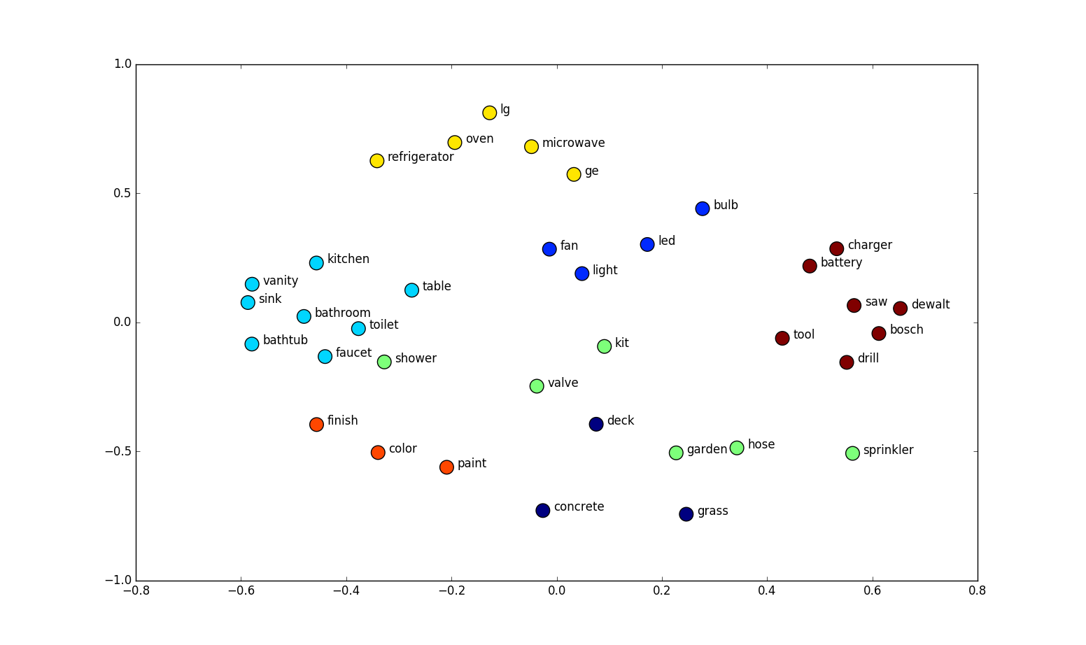
Word Embedding Visualization Analysis
The image displays a 2D scatter plot where words are positioned based on their semantic relationships. These positions derive from word embeddings that capture meaning based on context.
Key Word Clusters:
- Bathroom Fixtures: vanity, sink, toilet, bathtub, shower - grouped by their bathroom context
- Lighting: fan, light, bulb, led - connected through home lighting usage
- Tools: saw, dewalt, bosch, drill - associated with construction and hardware
- Home Finishing: finish, color, paint - related to decoration and renovation
- Outdoor/Gardening: deck, garden, hose, sprinkler, concrete - linked by outdoor usage
- Kitchen Appliances: oven, microwave, refrigerator, lg, ge - grouped as household appliances
This visualization demonstrates how word embeddings capture semantic relationships - nearby words share similar contexts, while distant words differ significantly in usage. The 2D representation efficiently reveals meaningful connections between terms that might appear in similar documents or discussions.
Word2Vec and The Skip-Gram Model: Core Concepts
Word2Vec changed how computers understand language by offering a fast way to learn word vectors from large amounts of text. These word vectors capture both meaning and grammar, allowing machines to grasp language more deeply. Word2Vec uses two main approaches: Continuous Bag-of-Words (CBOW) and Skip-gram. While CBOW predicts a target word based on its surrounding words, the Skip-gram model works the other way around—it uses a given word to predict its surrounding words. In this project, we focus on the Skip-gram model because it works very well with large datasets and can capture detailed relationships between words.
How Skip-Gram Works
The main goal of the Skip-gram model is to assign each word a unique vector such that, when placed in a vector space, words that often occur together end up close to each other, just like in the visualization above. To achieve this, the model examines a "window" around each target word. This window sets the number of words to the left and right that are considered its neighbors.
For each word in the text, the model chooses the target (center) word, examines the words that appear within a specified window around it, creates positive training pairs by pairing the target word with each neighboring word (labeled as 1) and finally, selects negative examples from words outside the window (labeled as 0).
By predicting the surrounding words for each target word, the model learns the context in which words are used. This process builds a deeper understanding of language, enabling the model to capture both the meaning and relationships between words. Ultimately, by the end of the training, each word is represented by a vector, and words that frequently appear together will occupy similar areas in the vector space.
Skip-gram Training Dataset Example
The Training Sentence
"Cats and dogs are popular pets while fish require less attention"
What's Happening Here
We're using this simple sentence to create training data for the Skip-gram model. The sentence is chosen because it:
- Uses common words that are easy to recognize.
- Naturally shows relationships between different types of pets.
- Contains a mix of nouns, verbs, adjectives, and connecting words.
- Has exactly 10 words, making it a clear and manageable example.
What We Intend to Do
For each word in this sentence, the Skip-gram model will:
- Select a target word: This is the word we focus on.
- Identify neighboring words: Look at the words within a set number of positions (called a window) around the target word.
- Create training pairs: Pair the target word with each of its neighbors. These pairs teach the model which words tend to appear together.
By doing this, the model learns the context in which each word appears.
Why Word2Vec Uses Both Positive and Negative Samples
When training Word2Vec, we want words that often appear together to have similar vector representations. To do this, we need two kinds of examples:
- Positive Samples: These are pairs of words that actually appear together in text.
- Negative Samples: These are pairs of words that do not appear together.
The Role of the Window
A "window" defines how many words on either side of a target word we consider. It sets the boundary for what counts as a neighboring word. Only words within this window are treated as context (and therefore become positive samples), while words outside the window are not considered related in that instance and can be used as negative samples.
Positive Samples
Consider the sentence:
"Cats and dogs are popular pets while fish require less attention"
If we choose "dogs" as our target word and set a window size of 2 that includes the two words before and after it, the words "and", "Cats", "are", and "popular" become positive samples. These are word pairs that naturally appear together, and we label these pairs with a 1. These examples help the model understand which words typically occur in the same context.
Negative Sampling
Negative samples serve as the counterbalance. They are examples of word pairs that do not appear together. For instance, if "cats" is the target word, words like "require", "attention", or "fish" (if they are not within the window) become negative samples, labeled with a 0. These negative examples force the model to differentiate between words that belong together and those that do not.
Why We Need Both Positive and Negative Samples
Imagine you're teaching a computer to tell the difference between apples and oranges. If you only show it apples, the computer will have no idea what makes an orange different. It might even decide that every fruit is an apple, because that’s all it has seen.
In Word2Vec training, positive samples show the computer which words go together. However, if we only use positive examples, the easiest solution for the model is to assign the same vector to every word. This minimizes errors, but it doesn’t capture any useful differences between words, just like calling every fruit an apple doesn't help in telling apples from oranges.
In Practice
When selecting negative samples, words are often chosen based on their frequency in the text. This adjustment helps avoid oversampling very common words while still providing a balanced set of examples. Together, positive and negative samples work like a push-pull system:
- Positive pairs pull related words closer together.
- Negative pairs push unrelated words apart.
This balance, along with the window that defines context, enables Word2Vec to create meaningful word embeddings that effectively capture both the similarities and differences between words.
Skip-gram Training Pairs
Using a window size of 2 (looking at 2 words on each side of the target word), here are all the positive training pairs generated:
| Window | Target Word (Main) | Context Word | Label |
|---|---|---|---|
| [Cats, and, ...] | Cats | and | 1 |
| [Cats, and, ...] | Cats | dogs | 1 |
| [..., Cats, and, dogs, ...] | and | Cats | 1 |
| [..., Cats, and, dogs, ...] | and | dogs | 1 |
| [..., Cats, and, dogs, ...] | and | are | 1 |
| [..., and, dogs, are, ...] | dogs | and | 1 |
| [..., and, dogs, are, ...] | dogs | Cats | 1 |
| [..., and, dogs, are, ...] | dogs | popular | 1 |
| [..., dogs, are, popular, ...] | are | dogs | 1 |
| [..., dogs, are, popular, ...] | are | and | 1 |
| [..., dogs, are, popular, ...] | are | pets | 1 |
| [..., are, popular, pets, ...] | popular | are | 1 |
| [..., are, popular, pets, ...] | popular | dogs | 1 |
| [..., are, popular, pets, ...] | popular | while | 1 |
| [..., popular, pets, while, ...] | pets | popular | 1 |
| [..., popular, pets, while, ...] | pets | are | 1 |
| [..., popular, pets, while, ...] | pets | fish | 1 |
| [..., pets, while, fish, ...] | while | pets | 1 |
| [..., pets, while, fish, ...] | while | popular | 1 |
| [..., pets, while, fish, ...] | while | require | 1 |
| [..., while, fish, require, ...] | fish | while | 1 |
| [..., while, fish, require, ...] | fish | pets | 1 |
| [..., while, fish, require, ...] | fish | less | 1 |
| [..., fish, require, less, ...] | require | fish | 1 |
| [..., fish, require, less, ...] | require | while | 1 |
| [..., fish, require, less, ...] | require | attention | 1 |
| [..., require, less, attention] | less | require | 1 |
| [..., require, less, attention] | less | fish | 1 |
| [..., require, less, attention] | less | attention | 1 |
| [..., less, attention] | attention | less | 1 |
| [..., less, attention] | attention | require | 1 |
Negative Sampling Examples
For each positive pair above, we would generate negative examples by randomly sampling words that aren't in the context window. Here are some negative sampling examples:
| Target Word (Main) | Context Word (Negative Sample) | Label |
|---|---|---|
| Cats | popular | 0 |
| Cats | fish | 0 |
| Cats | require | 0 |
| Cats | attention | 0 |
| dogs | fish | 0 |
| dogs | less | 0 |
| popular | Cats | 0 |
| popular | require | 0 |
| pets | Cats | 0 |
| pets | attention | 0 |
| fish | Cats | 0 |
| fish | dogs | 0 |
| fish | are | 0 |
| require | Cats | 0 |
| require | popular | 0 |
| attention | dogs | 0 |
| attention | popular | 0 |
| attention | while | 0 |
Complete Training Dataset (Sample)
Below is a sample of the complete training dataset combining both positive and negative examples:
| Target Word (Main) | Context Word | Label |
|---|---|---|
| Cats | and | 1 |
| Cats | dogs | 1 |
| Cats | popular | 0 |
| Cats | fish | 0 |
| and | Cats | 1 |
| and | dogs | 1 |
| and | are | 1 |
| and | fish | 0 |
| dogs | and | 1 |
| dogs | Cats | 1 |
| dogs | popular | 1 |
| dogs | fish | 0 |
| are | dogs | 1 |
| are | and | 1 |
| are | pets | 1 |
| are | attention | 0 |
| popular | are | 1 |
| popular | dogs | 1 |
| popular | while | 1 |
| popular | Cats | 0 |
| pets | popular | 1 |
| pets | are | 1 |
| pets | fish | 1 |
| pets | Cats | 0 |
| while | pets | 1 |
| while | popular | 1 |
| while | require | 1 |
| while | and | 0 |
| fish | while | 1 |
| fish | pets | 1 |
| fish | less | 1 |
| fish | Cats | 0 |
| require | fish | 1 |
| require | while | 1 |
| require | attention | 1 |
| require | are | 0 |
| less | require | 1 |
| less | fish | 1 |
| less | attention | 1 |
| less | dogs | 0 |
| attention | less | 1 |
| attention | require | 1 |
| attention | popular | 0 |
Main and Context Embeddings
In our training data, each word can appear in two roles: as a main (target) word and as a context word. The Skip-gram algorithm assigns a separate vector (or embedding) for each role, so every word ends up with two sets of embeddings:
- Main (Target) Embeddings: Used when the word is the focus or target of prediction. Think of this as the "identity" of the word. At the end of training, these are the embeddings we use to represent each word.
- Context Embeddings: Used when the word appears as part of the surrounding context of a target word. These capture how the word is used alongside other words.
At the beginning of training, both sets of embeddings are randomly assigned. Throughout training, they are updated based on the word's usage in different contexts. As we continue, we'll explain in detail how these two embeddings work together and how they are updated. For now, just remember that each word starts with two random embeddings, and together they help capture the full picture of word usage.
Imagine we start with two word embeddings for two different words, both randomly initialized at the beginning. We denote the main embeddings as M and the context embeddings as C.
For example: For the word "Cats", its main embedding might be: M = [2,2]. For the word "dogs", its context embedding might be: C = [5, -4]
These values are chosen at random before training begins, and they will be updated as the model learns from the text.
Cats and Dog vector space viz
From our training data, we know that the pair (cats, dogs) has a label of 1, meaning that these words appear together in similar contexts. Our goal is to have the model learn embeddings so that words that often occur together are placed near each other in the vector space.
In this process, we start with randomly initialized embeddings and update them during training. Consider the following initializations (as shown in the graph):
- Main word "cats" has a vector M = [2, 2]
- Context word "dogs" has a vector C = [5, -4]
Dot Product: Measuring Similarity
The dot product of two vectors is a simple way to measure their similarity. It gives a single number that tells us whether the vectors point in a similar direction. In our context, a larger dot product indicates that the words are more similar (i.e., they occur in similar contexts), while a smaller or negative dot product suggests they are not.
Let's calculate the dot product for our example:
$$ \text{Dot Product} = (2 \times 5) + (2 \times -4) = 10 - 8 = 2 $$
Converting the Dot Product to a Probability with the Sigmoid Function
The raw dot product (in our case, 2) can be any real number, which isn't directly interpretable as a probability. Since Word2Vec borrows ideas from logistic regression for its training (a binary classification problem), we need to convert this raw score into a value between 0 and 1.
The sigmoid function does exactly that. It is defined as:
$$ \sigma(x) = \frac{1}{1 + e^{-x}} $$
Applying the sigmoid function to our dot product:
$$ \sigma(2) = \frac{1}{1 + e^{-2}} \approx \frac{1}{1 + 0.1353} \approx \frac{1}{1.1353} \approx 0.88 $$
A sigmoid output of 0.88 means that, according to the current embeddings, there is a high probability (close to 1) that the words "cats" (as a main word) and "dogs" (as a context word) occur together. This aligns with our training label of 1.
Why This Process Is Important
- Measuring Similarity: The dot product gives us a raw measure of how similar two embeddings are.
- Probability Interpretation: The sigmoid function transforms that raw score into a probability between 0 and 1. A value near 1 indicates that the model predicts the pair appears together (a positive sample), while a value near 0 would indicate they do not.
- Training with Binary Labels: Since Word2Vec treats the prediction task as a binary classification (using logistic regression), this probability is compared with the actual label (1 for words that appear together and 0 for those that do not). The difference between the prediction and the label is used to update the embeddings during training which we will talk about later on.
In summary, we calculate the dot product to get a raw similarity score between the main and context embeddings, and then apply the sigmoid function to convert this score into a probability.
The next step is to calculate another vector called the difference vector (or "diffs"). This is done by subtracting the main embedding from the context embedding:
$$ \text{diffs} = \text{Context} - \text{Main} $$
Using our example:
- Main vector for "cats": [2, 2]
- Context vector for "dogs": [5, -4]
The difference vector is calculated as:
$$ \text{diffs} = [5, -4] - [2, 2] = [3, -6] $$
Difference Vector: A Guide for Updates
Knowing how similar two vectors are (via the dot product) tells us their current relationship, but it doesn't say how to adjust them during training. That’s where the difference vector comes in, it acts like a roadmap for updates:
- Bridging the Gap: If the main vector (\(\mathbf{v}_{\text{center}}\)) needs to become more like the context vector (\(\mathbf{w}_{\text{context}}\)), you adjust it in the direction of the difference vector.
- Pushing Apart: Conversely, if the model needs the vectors to be less similar (for negative samples), you update the main vector in the opposite direction.
Think of the difference vector as giving you exact directions—how many steps and in which direction (left/right, up/down) you need to move each element of the vector to bring them closer together or push them further apart.
In our analogy, if you and a friend are trying to meet, the dot product tells you you're heading generally in the same direction, but the difference vector tells you exactly how many steps each of you needs to take to meet exactly in the middle.
Thus, the difference vector is key to guiding the adjustments during training. It provides precise instructions on how to tweak the embeddings so that similar words get closer together, while dissimilar words are pushed apart.
Difference Vector
From the graph above, we see a difference vector in addition to the main and context vectors. The difference vector is simply what you get when you subtract the main vector from the context vector. It tells you, for each part of the vector, how much they differ. In other words, it shows exactly how much each element in the main vector should be changed to match the context vector. During training, this difference guides the adjustments made to the embeddings. The difference line is a visual representation of the gap between the main and context vectors. It’s a line drawn from the main vector to the context vector that shows both the direction and the distance between them. Think of it as a roadmap that indicates which way the main vector should move to get closer to the context vector, and vice versa.
Computing the Error
For each pair \((\mathbf{main}, \mathbf{context})\), the model calculates an error value that tells us how much the prediction is off. Here's how we do it:
-
Predict the Similarity: First, compute the dot product of the main and context vectors. Then, apply the sigmoid function to the dot product to convert it into a probability \(\hat{y}\) (a number between 0 and 1).
-
Compare to the True Label: Each pair has a true label, \(y\), where \(y = 1\) if it's a real (positive) pair and \(y = 0\) if it's a negative pair. In our scenario, we have a true label of 1. The error is calculated by subtracting the predicted probability from the true label: $$ \text{Error} = y - \hat{y} $$
-
Example Calculation:
The dot product gave us a similarity of 0.88 for the cats (main) and dog (context) embeddings. Then, the error is: $$ \text{Error} = 1 - 0.88 = 0.12 $$ A larger error indicates that the prediction was far off from the true value, signaling a need for a bigger adjustment during training. A smaller error, as in our scenario, indicates that we weren't too far off from the true value. Our initial randomization was pretty good. This error will essentially guide how much and in what direction we update the embeddings.
Applying Updates
After computing the error between the predicted similarity and the true label, we update both the main and context embeddings so that they better reflect each other's influence. The process involves calculating a difference vector, scaling it according to the error and learning rate, and then applying the updates in opposite directions to the two embeddings. Here's how it works:
-
Calculate the Difference Vector (Diffs):
The difference vector is the element-wise difference between the context and main embeddings: $$ \text{Diffs} = \text{Context} - \text{Main} $$ For example, if the Main Embedding is \([2, 2]\) and the Context Embedding is \([5, -4]\), then: $$ \text{Diffs} = [5, -4] - [2, 2] = [3, -6] $$ -
Scale the Difference Vector:
The update is determined by three factors:- Diffs: Provides the direction to move.
- Error: Indicates how far off the prediction is.
- Learning Rate: Controls the size of the update step.
The update vector is computed as: $$ \text{Update} = \text{Diffs} \times \text{Error} \times \text{Learning Rate} $$ For instance, if our error is \(0.12\) and we choose a learning rate of \(0.1\), then the scale factor is: $$ \text{Scale Factor} = 0.12 \times 0.1 = 0.012 $$ Multiplying the difference vector by this scale factor gives: $$ \text{Update} = [3, -6] \times 0.012 = [0.036, -0.072] $$
- Apply the Update:
The updates are applied in opposite directions: - Main Embedding:
Move the main embedding toward the context embedding by adding the update vector: $$ \text{Main}_{\text{new}} = \text{Main}_{\text{old}} + \text{Update} $$ For our example: $$ \text{Main}_{\text{new}} = [2, 2] + [0.036, -0.072] = [2.036, 1.928] $$ - Context Embedding:
Simultaneously, move the context embedding toward the main embedding by subtracting the update vector: $$ \text{Context}_{\text{new}} = \text{Context}_{\text{old}} - \text{Update} $$ For our example: $$ \text{Context}_{\text{new}} = [5, -4] - [0.036, -0.072] = [4.964, -3.928] $$
Intuitive Summary
-
Difference Vector (Diffs):
Acts as a roadmap, showing the direction and distance from the main embedding to the context embedding. -
Error:
Quantifies how far off the prediction is; a larger error calls for a bigger correction. -
Learning Rate:
Controls the magnitude of the adjustment, ensuring that updates are gradual and stable.
By multiplying these factors: $$ \text{Update} = \text{Diffs} \times \text{Error} \times \text{Learning Rate} $$ we obtain an update vector that retains the direction of the difference vector but is scaled to a small, controlled step.
Moving the main and context embeddings in opposite directions is important because it ensures that both sets of embeddings are adjusted in a way that minimizes the overall error. Think of it like two sides of the same coin—both need to be adjusted to better match each other. Here's why:
-
Balanced Adjustment:
By updating the main embedding toward the context embedding and vice versa, you're effectively reducing the gap between them. This balanced adjustment helps the model learn a more accurate representation of how words co-occur. If only one side was updated, you might end up with an imbalance where one embedding overcompensates while the other remains fixed. -
Error Minimization:
This process is similar to backpropagation in neural networks. In backpropagation, you calculate the error (or gradient) and then adjust the weights in the network to minimize that error. Here, the error tells us how "wrong" our prediction was, and by updating both embeddings appropriately, we are reducing that error. Each update moves the embeddings a little bit closer (or further apart) in the direction needed to improve the model's prediction. -
Symmetric Learning:
When both embeddings are updated, they "pull" each other toward a common representation that reflects their true contextual relationship. This mutual adjustment is essential for creating a well-organized vector space where similar words are close together.
Thus, updating both the main and context embeddings in opposite directions is akin to the error-minimization process in backpropagation. It ensures that every pair of embeddings is fine-tuned based on the error signal, leading to more accurate and meaningful word representations.
This symmetric update process gradually shapes the embedding space over many training iterations, ensuring that words with similar contexts are drawn together while words with different contexts are pushed apart. In essence, the process uses the error to determine the magnitude of change, the difference vector to set the direction, and the learning rate to control the step size, thereby fine-tuning the word embeddings.
Visualizing Main and Context Updates
This plot visualizes how the update process works for two word embeddings using simple vector math:
-
M (Main Vector):
The original main embedding is shown at the point (2, 2) and labeled "M" in blue. -
C (Context Vector):
The original context embedding is shown at the point (5, -4) and labeled "C" in red. -
D (Difference Vector):
The dashed green line labeled "D (C - M)" connects M to C. This line represents the difference between the context and main embeddings, indicating the direction and distance needed to move from M to C. -
M' (Updated Main Vector):
After applying the update, the main embedding shifts to a new position at (2.5, 1). This updated position is labeled "M'" and is still shown in blue. -
C' (Updated Context Vector):
Simultaneously, the context embedding moves toward the main embedding and ends up at (4.5, -3). This updated context embedding is labeled "C'" and is shown in red. -
M' Arrow (Main Update Arrow):
A solid orange arrow is drawn from the original main embedding (M) to its new position (M'). This arrow shows the direction and magnitude of the update applied to the main vector. -
C' Arrow (Context Update Arrow):
Similarly, a solid orange arrow is drawn from the original context embedding (C) to its updated position (C'). This arrow indicates how the context vector is adjusted in the opposite direction.
The plot demonstrates that the main and context embeddings are adjusted based on their difference, they are updated in opposite directions (M moves toward C, and C moves toward M), reducing the gap between them, and the difference vector (dashed green line) guides the update, and the update arrows (orange) visually show the adjustments made to each vector.
Putting it all together
What we went over considered one main word and one context word. In reality, the main word gets influenced by multiple context words. Now, let's go back to the sentence we used to generate the training data to see how this happens.
"Cats and dogs are popular pets while fish require less attention."
We'll focus on how the word "fish" is updated during training. Suppose the current main embedding for "fish" is: $$ [3.0,\, 1.0] $$
Two Ways to Update the Word Embedding
1. Sequential Updates (Common in Skip-gram)
Assume that in the sentence "Cats and dogs are popular pets while fish require less attention," the word "fish" appears with several context words. For this example, let’s say it appears with three context words: "require," "less," and "attention." For each of these, we compute an update value that nudges the embedding of "fish."
  Update from "require": +0.014
  Update from "less": +0.021
  Update from "attention": +0.132
We then apply these updates one after the other to the current main embedding:
- Update with "require":
$$ \text{New embedding} = [3.0,\, 1.0] + [0.014,\, 0.014] = [3.014,\, 1.014] $$ - Update with "less":
$$ \text{New embedding} = [3.014,\, 1.014] + [0.021,\, 0.021] = [3.035,\, 1.035] $$ - Update with "attention":
$$ \text{New embedding} = [3.035,\, 1.035] + [0.132,\, 0.132] = [3.167,\, 1.167] $$
Thus, after sequential updates, the final embedding for "fish" becomes: $$ [3.167,\, 1.167] $$
2. Batch Updates (Common in Larger Systems)
Alternatively, we can accumulate all updates and apply them at once:
- Calculate the Total Update: $$ \text{total_update} = [0.014,\, 0.014] + [0.021,\, 0.021] + [0.132,\, 0.132] = [0.167,\, 0.167] $$
- Apply the Total Update: $$ \text{New embedding} = [3.0,\, 1.0] + [0.167,\, 0.167] = [3.167,\, 1.167] $$
Both approaches yield the same final result, but in the batch method, the vector is updated only once.
Why Word Embeddings Cluster by Meaning
After training on millions of sentences, each word's main embedding settles into a position that reflects all of its contexts. For example, the main embedding for "fish" is influenced by the context words it appears with (such as "require," "less," "attention," and possibly others like "water" or "ocean" from different sentences). Simultaneously, when "fish" acts as a context word, it pulls other main embeddings toward itself.
Over many training iterations:
- Similar words share many of the same context words, so they receive similar updates and end up clustered together.
- Words with different meanings form distinct clusters.
- Relationships between words emerge as consistent vector differences, enabling analogies such as: $$ \text{king} - \text{man} + \text{woman} \approx \text{queen} $$
This clustering happens naturally from the statistical patterns in language without any explicit semantic rules.
What's Actually Happening in Each Update
-
Direction:
The update moves the main word embedding toward (or away from) the context word embedding. The difference vector, calculated as \( \text{Context} - \text{Main} \), provides the direction. -
Magnitude:
Each update's size is scaled by an error term and a learning rate. If the model's prediction is already close to the true label, the update is small; the learning rate ensures that changes happen gradually. -
Multiple Updates:
In real text, "fish" appears with many context words. Positive pairs (e.g., "fish"-"water") pull the embedding together, while negative pairs (e.g., "fish"-"algebra") push it apart. The final position of "fish" is the cumulative result of all these small updates. -
Vector Transformation:
As a consequence, words with similar contexts end up with similar vector representations, forming a meaningful semantic space.
Context Embeddings Also Update
To recap, Word2Vec uses two sets of embeddings: Main (Center) Word Embeddings which represent the target words and Context Word Embeddings which represent the surrounding words.
During each training step: - The main embedding for "fish" is updated by adding the update vector (moving it toward its context words). - The corresponding context embeddings are updated by subtracting the update vector (moving them in the opposite direction).
This opposing update mechanism:
  - Prevents words from collapsing into a single point.
  - Creates a balanced "tug-of-war" dynamic where words that frequently appear together are drawn close, but still maintain distinct positions.
In many implementations, only the main embeddings are used for downstream tasks; however, some systems combine both.
Thus, continuous, small adjustments cause words with similar contexts to cluster together, while different words settle into distinct regions. This emergent property of the Word2Vec algorithm creates a rich semantic space where relationships between words are captured through simple vector arithmetic.
import torch
import torch.nn.functional as F  # For activation functions like sigmoid and normalization
import numpy as np
import pandas as pd
import string
from tqdm import tqdm
from scipy.spatial.distance import cosine
import matplotlib.pyplot as plt

# -----------------------------
# Data Preprocessing
# -----------------------------
# Load stopwords from file and split into a list
with open('stopwords.txt') as f:
    stopwords = f.read().replace('\n', ' ').split()

# Read the training text from file (assumed to be a single large text block)
with open('training_text.txt', encoding='utf-8') as f:
    text = f.read().replace('\n', '')
    print(text)  # Print the raw text for verification
    # Remove punctuation from the text
    text = text.translate(str.maketrans('', '', string.punctuation))
    # Remove digits from the text
    text = ''.join([t for t in text if t not in list('0123456789')])
    # Remove special quote characters, convert text to lower case, and split into words
    text = text.replace('”', '').replace('“', '').replace('’', '').lower().split()

# Remove stopwords and limit the number of words for speed (e.g., use the first 2000 words)
text = [w for w in text if w not in stopwords][:2000]

# -----------------------------
# Build Training Data
# -----------------------------
WINDOW_SIZE = 3           # Number of words to consider on either side of the center word
NUM_NEGATIVE_SAMPLES = 3  # Number of negative samples to generate per positive pair

data = []

# Build training pairs: for each center word, pair it with context words
# Then add negative samples (words not in the context) with label 0
for idx, center_word in enumerate(text[WINDOW_SIZE-1:-WINDOW_SIZE]):
    # Define the context: words in a window around the center word
    context_words = [w for w in text[idx:idx+2*WINDOW_SIZE-1] if w != center_word]

    for context_word in context_words:
        # Positive example: center word with a context word that appears in its window
        data.append([center_word, context_word, 1])

        # Negative sampling: choose words that are not the center or in its context window
        negative_samples = np.random.choice(
            [w for w in text[WINDOW_SIZE-1:-WINDOW_SIZE] if w != center_word and w not in context_words],
            NUM_NEGATIVE_SAMPLES
        )
        for neg in negative_samples:
            # Negative example: label is 0
            data.append([center_word, neg, 0])

# Create a DataFrame from the training pairs
df = pd.DataFrame(columns=['center_word', 'context_word', 'label'], data=data)
# Only use words that appear as both center and context for consistency
words = np.intersect1d(df.context_word, df.center_word)
df = df[(df.center_word.isin(words)) & (df.context_word.isin(words))].reset_index(drop=True)

# -----------------------------
# Create Vocabulary and Mapping
# -----------------------------
# Build the vocabulary (sorted list of unique words)
vocab = sorted(set(words))
# Create a mapping from each word to a unique index
word_to_index = {word: idx for idx, word in enumerate(vocab)}
vocab_size = len(vocab)

# -----------------------------
# Initialize Embeddings as PyTorch Tensors
# -----------------------------
EMBEDDING_SIZE = 5  # Dimensionality of the embeddings

# Initialize main embeddings with random normal values and scale them by 0.1
main_embeddings = torch.randn(vocab_size, EMBEDDING_SIZE) * 0.1
# Normalize each embedding vector to have unit length (L2 normalization)
main_embeddings = F.normalize(main_embeddings, p=2, dim=1)

# Similarly, initialize context embeddings
context_embeddings = torch.randn(vocab_size, EMBEDDING_SIZE) * 0.1
context_embeddings = F.normalize(context_embeddings, p=2, dim=1)

# -----------------------------
# Update Function using PyTorch
# -----------------------------
def update_embeddings(df, main_embeddings, context_embeddings, learning_rate):
    """
    For each training pair (center, context) in the DataFrame df, update the main and context embeddings.
    The update is computed based on the difference between the context and main embeddings,
    scaled by the prediction error and the learning rate.

    Parameters:
    - df: DataFrame containing training pairs with columns ['center_word', 'context_word', 'label']
    - main_embeddings: PyTorch tensor of main word embeddings (size: vocab_size x EMBEDDING_SIZE)
    - context_embeddings: PyTorch tensor of context word embeddings (size: vocab_size x EMBEDDING_SIZE)
    - learning_rate: scalar controlling the update magnitude

    Returns:
    - Updated main_embeddings and context_embeddings as PyTorch tensors.
    """
    # Initialize update accumulators for main and context embeddings
    main_updates = torch.zeros_like(main_embeddings)
    context_updates = torch.zeros_like(context_embeddings)

    # Loop over each training example (can be vectorized for performance)
    for i, row in df.iterrows():
        center_word = row['center_word']
        context_word = row['context_word']
        label = row['label']

        # Retrieve indices for the current center and context words
        center_idx = word_to_index[center_word]
        context_idx = word_to_index[context_word]

        # Get the embeddings for the center and context words
        main_vec = main_embeddings[center_idx]       # Main embedding for center word
        context_vec = context_embeddings[context_idx] # Context embedding for context word

        # Compute the difference vector: how far the context embedding is from the main embedding
        diff = context_vec - main_vec

        # Compute similarity via dot product
        dot_prod = torch.dot(main_vec, context_vec)
        # Apply sigmoid to convert the dot product into a probability (score between 0 and 1)
        score = torch.sigmoid(dot_prod)

        # Compute error: the difference between the true label and the predicted score
        error = label - score  # This is a scalar value

        # Compute the update vector: scale the difference by error and learning rate
        update = diff * error * learning_rate

        # Accumulate the updates:
        # For the main embedding, add the update vector (moving it toward the context embedding)
        main_updates[center_idx] += update
        # For the context embedding, subtract the update vector (moving it in the opposite direction)
        context_updates[context_idx] += update

    # Apply the accumulated updates to the embeddings
    main_embeddings = main_embeddings + main_updates
    context_embeddings = context_embeddings - context_updates

    # Normalize the updated embeddings to maintain unit length
    main_embeddings = F.normalize(main_embeddings, p=2, dim=1)
    context_embeddings = F.normalize(context_embeddings, p=2, dim=1)

    return main_embeddings, context_embeddings

# -----------------------------
# Training Loop
# -----------------------------
num_epochs = 25
learning_rate = 0.1

# Run through multiple epochs of updating embeddings
for epoch in range(num_epochs):
    main_embeddings, context_embeddings = update_embeddings(df, main_embeddings, context_embeddings, learning_rate)
    print(f"Epoch {epoch+1}/{num_epochs} completed.")

# -----------------------------
# Compute Similarities between Words (Using Cosine Similarity)
# -----------------------------
results = []
# Loop over every pair of words in the vocabulary
for w1 in vocab:
    for w2 in vocab:
        if w1 != w2:
            idx1, idx2 = word_to_index[w1], word_to_index[w2]
            # Compute cosine similarity between the main embeddings of w1 and w2
            sim = 1 - cosine(main_embeddings[idx1].detach().numpy(), main_embeddings[idx2].detach().numpy())
            results.append((w1, w2, sim))

# For demonstration, sort and print the top 10 most similar words to a given word, e.g., "town"
similarities_for_town = sorted([item for item in results if item[0] == 'town'], key=lambda t: -t[2])[:10]
print(similarities_for_town)
In this article, we explored how Word2Vec learns word representations by training on a simple natural language data.
Comments (0)