In our previous article, we discussed the skip-gram word2vec approach. The skip-gram model predicts context words given a target or central word. It learns through training data that labels words within a specified window as 1 and distant words as 0. The model compares main embeddings and context embeddings, updating them to increase cosine similarity (or dot product) for positive pairs while pushing negative examples further apart. Through iterative updates, embeddings of related words gradually converge, while those of unrelated words diverge, yielding a semantic space where proximity reflects linguistic similarity.

Motivation for a New Approach

What if we wish to create embeddings that reflect a continuous outcome rather than simple co-occurrence? Consider applications in which words are meant to capture their impact on external metrics, such as the pricing of products, stock performance, or customer sentiment intensity, rather than solely their contextual usage. With this in mind, we propose ValueVec, a variant of word2vec where word similarity aligns with an external value, such as price.

Our objective is to represent words in a vector space so that the distance or similarity between their embeddings reflects the degree of similarity in their value impacts. In other words, words with similar impacts (whether that similarity is represented by high or low cosine similarity) are mapped closer together, and those with dissimilar impacts are positioned further apart. Crucial to this approach is the meticulous construction of training data that captures these value differences.

The Value-Driven Approach

Traditional word2vec models rely on linguistic context alone, where words appearing together yield similar embeddings. In contrast, our ValueVec implementation incorporates an external continuous value (like price) to define word relationships.

Key features of our ValueVec implementation:

• Value-Based Similarity:
  Words are considered similar if they have similar impacts on a continuous label, not merely because they co-occur.

• Continuous Target Labels:
  Unlike binary labels in the original word2vec (1 for context words, 0 for negatives), we use continuous labels (normalized between 0 and 1) to indicate the degree of similarity based on external metrics.

• Enhanced Negative Sampling:
  Negative samples are selected based on notably different external values, enforcing more meaningful contrasts in the embedding space.

• Direct Optimization:
  The training objective is modified to directly adjust the cosine similarity of word embeddings to match the target continuous scores.

These changes create an embedding space where, for example, keywords with similar price impacts or market influences naturally group together.

Applications

This value-sensitive embedding technique has several practical applications:

1. E-commerce Keyword Optimization:
   Identifying keywords with similar price impacts to improve product listing strategies.

2. Investment Analysis:
   Clustering terms in financial reports by their correlation with stock performance.

3. Customer Segmentation:
   Grouping descriptors based on their association with customer lifetime value.

4. Sentiment Analysis:
   Developing nuanced embeddings that capture the intensity of emotions, not just simple polarity.

By explicitly incorporating external metrics into our word embeddings, ValueVec creates representations that are better aligned with specific business objectives and quantitative outcomes.

def create_color_spectrum_dataset(n_colors=20, random_seed=42):
    """
    Create a simple dataset of colors positioned along the visible light spectrum.
    
    Args:
        n_colors: Number of colors to generate
        random_seed: Random seed for reproducibility
    
    Returns:
        DataFrame with color names and their position values (wavelength)
        vocabulary: List of all unique color names
    """
    # Set random seed for reproducibility
    random.seed(random_seed)
    np.random.seed(random_seed)
    
    # Base colors in spectrum order (roughly corresponding to wavelength)
    base_colors = [
        "violet", "indigo", "blue", "cyan", "teal", "green", 
        "chartreuse", "yellow", "gold", "orange", "red", "crimson"
    ]
    
    # Generate derived color names by adding modifiers
    modifiers = ["light", "dark", "vivid", "pale", "deep", "bright"]
    
    colors = base_colors.copy()
    while len(colors) < n_colors:
        base = random.choice(base_colors)
        modifier = random.choice(modifiers)
        new_color = f"{modifier}-{base}"
        if new_color not in colors:
            colors.append(new_color)
    
    # Trim to exact number requested
    colors = colors[:n_colors]
    
    # Assign positions along the spectrum (wavelength in nm, approximately)
    # Violet ~380nm to Red ~750nm
    base_positions = {
        "violet": 380,
        "indigo": 420,
        "blue": 460,
        "cyan": 490,
        "teal": 510,
        "green": 530,
        "chartreuse": 560,
        "yellow": 580,
        "gold": 600,
        "orange": 620,
        "red": 680,
        "crimson": 730
    }
    
    # Function to get position, adding small noise for modifiers
    def get_position(color):
        if color in base_positions:
            return base_positions[color]
        else:
            # For derived colors, extract the base
            parts = color.split('-')
            modifier = parts[0]
            base = parts[1]
            
            base_pos = base_positions[base]
            
            # Modifiers shift the position slightly
            modifier_shifts = {
                "light": -10,
                "dark": +10,
                "vivid": -5,
                "pale": -15,
                "deep": +15,
                "bright": -8
            }
            
            shift = modifier_shifts.get(modifier, 0)
            # Add a small random noise
            noise = np.random.normal(0, 3)
            
            return base_pos + shift + noise
    
    # Create the dataset
    df = pd.DataFrame({
        "keyword": colors,
        "estimated_value": [get_position(color) for color in colors]
    })
    
    # Sort by wavelength to see the spectrum order
    df = df.sort_values("estimated_value").reset_index(drop=True)
    
    # Create vocabulary list
    vocabulary = df["keyword"].tolist()
    
    print(f"Created dataset with {len(df)} colors along the visible spectrum")
    print(df.head())
    
    return df, vocabulary

This code generates a reproducible synthetic dataset where each color name is associated with a numerical value representing its position on the visible spectrum. It uses a combination of base colors and modifiers to increase the diversity of the dataset and then applies a function to assign a realistic wavelength value to each color name. This dataset serves as an illustrative example for experiments, such as clustering or embedding in vector spaces based on continuous values. The table below is the data it generated.

keyword	estimated_value
light-violet	368.591577
bright-violet	371.585207
violet	380.000000
indigo	420.000000
dark-indigo	431.627680
blue	460.000000
cyan	490.000000
light-teal	500.942742
deep-cyan	503.609747
dark-cyan	504.569090
teal	510.000000
dark-teal	521.943066
green	530.000000
chartreuse	560.000000
dark-chartreuse	568.313137
yellow	580.000000
deep-yellow	591.961507
light-gold	594.737638
gold	600.000000
pale-orange	607.302304
light-orange	608.602811
dark-gold	610.725887
orange	620.000000
bright-red	671.297589
light-red	671.490142
red	680.000000
bright-crimson	716.260159
light-crimson	719.297540
crimson	730.000000
deep-crimson	739.825247

The Visible Spectrum and Estimated Values

The visible spectrum is the portion of the electromagnetic spectrum that the human eye can perceive. It ranges from about 380 nanometers (violet) to about 750 nanometers (red). In everyday terms, it’s the range of colors you see in a rainbow: violet, blue, green, yellow, orange, and red.

In this context, the estimated_value represents the approximate position of a color along the visible spectrum, measured in nanometers. For base colors, fixed wavelength values are used (for example, violet is around 380 nm). For derived colors with modifiers (like "light-violet" or "dark-indigo"), these base values are adjusted by applying a shift based on the modifier and adding a small amount of random noise to simulate natural variability.

In simple terms, the estimated_value shows where a color falls along the spectrum—from shorter wavelengths (violet) to longer wavelengths (red). The objective is to embed these colors into a vector space such that colors with similar wavelengths, hence similar positions along the visible spectrum—are clustered together. This means that colors sharing close estimated wavelengths (for example, various shades of violet) would be positioned near one another, reflecting their natural ordering and perceptual similarity.

import torch
import torch.nn.functional as F
import pandas as pd
import random

def create_color_training_pairs(df, context_window_size=2, num_negatives=5):
    """
    Create training pairs with more negative examples and non-linear similarity.
    
    Args:
        df: DataFrame with keywords and estimated_price.
        context_window_size: Number of words before/after to use as positive pairs.
        num_negatives: Number of negative samples per center word.
    
    Returns:
        train_df: DataFrame with training pairs and labels.
        vocabulary: List of all unique keywords.
        sorted_df: DataFrame sorted by price.
    """
    # Normalize the price values
    max_price = df["estimated_value"].max()
    min_price = df["estimated_value"].min()
    df["normalized_value"] = (df["estimated_value"] - min_price) / (max_price - min_price)
    
    # Sort DataFrame by price descending
    sorted_df = df.sort_values(by="estimated_value", ascending=False).reset_index(drop=True)
    
    center_words = []
    context_words = []
    labels = []
    center_values = []
    context_values = []
    pair_types = []
    
    n = len(sorted_df)
    vocabulary = sorted_df["keyword"].tolist()
    
    # Calculate minimum distance for negative sampling (25% of vocabulary size)
    min_distance = max(1, int(n * 0.25))
    
    for i in range(n):
        center_word = vocabulary[i]
        center_value = sorted_df.iloc[i]["normalized_value"]
        
        # Positive pairs: nearby words
        for j in range(1, context_window_size + 1):
            # Words before the center word
            if i - j >= 0:
                context_word = vocabulary[i - j]
                context_value = sorted_df.iloc[i - j]["normalized_value"]
                center_words.append(center_word)
                context_words.append(context_word)
                
                # Non-linear similarity (sharper drop-off for differences)
                diff = abs(center_value - context_value)
                similarity = max(0, 1.0 - (diff * 2.0)**2)  # Quadratic penalty
                
                labels.append(similarity)
                center_values.append(center_value)
                context_values.append(context_value)
                pair_types.append("positive")
            
            # Words after the center word
            if i + j < n:
                context_word = vocabulary[i + j]
                context_value = sorted_df.iloc[i + j]["normalized_value"]
                center_words.append(center_word)
                context_words.append(context_word)
                
                # Non-linear similarity (sharper drop-off for differences)
                diff = abs(center_value - context_value)
                similarity = max(0, 1.0 - (diff * 2.0)**2)  # Quadratic penalty
                
                labels.append(similarity)
                center_values.append(center_value)
                context_values.append(context_value)
                pair_types.append("positive")
        
        # Multiple negative pairs with emphasis on extremes
        neg_indices = []
        
        # Add furthest word as guaranteed negative
        furthest_idx = 0 if i > n/2 else n-1
        neg_indices.append(furthest_idx)
        
        # Add more random distant words
        remaining_negatives = num_negatives - 1
        
        # Define distant indices (words at least min_distance away)
        distant_indices = list(range(0, max(0, i-min_distance))) + list(range(min(n-1, i+min_distance), n))
        
        if distant_indices and remaining_negatives > 0:
            # Sample without replacement if possible
            sample_size = min(remaining_negatives, len(distant_indices))
            sampled_indices = random.sample(distant_indices, sample_size)
            neg_indices.extend(sampled_indices)
        
        for neg_idx in neg_indices:
            context_word = vocabulary[neg_idx]
            context_value = sorted_df.iloc[neg_idx]["normalized_value"]
            center_words.append(center_word)
            context_words.append(context_word)
            
            # Even more aggressive penalty for negative examples
            diff = abs(center_value - context_value)
            similarity = max(0, 1.0 - diff * 3.0)  # Linear but steeper penalty
            
            labels.append(similarity)
            center_values.append(center_value)
            context_values.append(context_value)
            pair_types.append("negative")
    
    # Create DataFrame with all training pairs
    train_df = pd.DataFrame({
        "center_word": center_words,
        "context_word": context_words,
        "label": labels,
        "center_value": center_values,
        "context_value": context_values,
        "pair_type": pair_types
    })

First 20 Rows of Training Data

Index	Center Word	Context Word	Label	Center Value	Context Value	Pair Type
0	deep-crimson	crimson	0.997198	1.000000	0.973534	positive
1	deep-crimson	light-crimson	0.987769	1.000000	0.944704	positive
2	deep-crimson	light-violet	0.000000	1.000000	0.000000	negative
3	deep-crimson	light-gold	0.000000	1.000000	0.609174	negative
4	deep-crimson	light-violet	0.000000	1.000000	0.000000	negative
5	crimson	deep-crimson	0.997198	0.973534	1.000000	positive
6	crimson	light-crimson	0.996675	0.973534	0.944704	positive
7	crimson	bright-crimson	0.994521	0.973534	0.936522	positive
8	crimson	light-violet	0.000000	0.973534	0.000000	negative
9	crimson	deep-cyan	0.000000	0.973534	0.363701	negative
10	crimson	dark-teal	0.000000	0.973534	0.413086	negative
11	light-crimson	crimson	0.996675	0.944704	0.973534	positive
12	light-crimson	bright-crimson	0.999732	0.944704	0.936522	positive
13	light-crimson	deep-crimson	0.987769	0.944704	1.000000	positive
14	light-crimson	red	0.955178	0.944704	0.838847	positive
15	light-crimson	light-violet	0.000000	0.944704	0.000000	negative
16	light-crimson	green	0.000000	0.944704	0.434789	negative
17	light-crimson	deep-yellow	0.000000	0.944704	0.601696	negative
18	bright-crimson	light-crimson	0.999732	0.936522	0.944704	positive
19	bright-crimson	red	0.961839	0.936522	0.838847	positive

---

Last 20 Rows of Training Data

Index	Center Word	Context Word	Label	Center Value	Context Value	Pair Type
184	indigo	light-red	0.000000	0.138480	0.815924	negative
185	indigo	yellow	0.000000	0.138480	0.569475	negative
186	violet	indigo	0.953561	0.030731	0.138480	positive
187	violet	bright-violet	0.997945	0.030731	0.008064	positive
188	violet	dark-indigo	0.922637	0.030731	0.169802	positive
189	violet	light-violet	0.996222	0.030731	0.000000	positive
190	violet	deep-crimson	0.000000	0.030731	1.000000	negative
191	violet	light-gold	0.000000	0.030731	0.609174	negative
192	violet	dark-gold	0.000000	0.030731	0.652242	negative
193	bright-violet	violet	0.997945	0.008064	0.030731	positive
194	bright-violet	light-violet	0.999740	0.008064	0.000000	positive
195	bright-violet	indigo	0.931967	0.008064	0.138480	positive
196	bright-violet	deep-crimson	0.000000	0.008064	1.000000	negative
197	bright-violet	dark-cyan	0.000000	0.008064	0.366286	negative
198	bright-violet	green	0.000000	0.008064	0.434789	negative
199	light-violet	bright-violet	0.999740	0.000000	0.008064	positive
200	light-violet	violet	0.996222	0.000000	0.030731	positive
201	light-violet	deep-crimson	0.000000	0.000000	1.000000	negative
202	light-violet	orange	0.000000	0.000000	0.677224	negative
203	light-violet	deep-cyan	0.000000	0.000000	0.363701	negative

Explanation of Training Data Columns

• center_word:
  The anchor or reference word in the pair — the word for which similarity relationships are being modeled.

• context_word:
  The word being compared to the center_word. In positive pairs, it appears within a defined context window; in negative pairs, it’s sampled from words farther apart in the sorted list.

• label:
  A numerical similarity score between center_word and context_word.

• For positive pairs, the score is computed using a quadratic penalty that drops sharply as the difference in values increases.

• For negative pairs, the score is computed using a linear penalty to aggressively reduce similarity for items with large value differences.

• center_value:
  The normalized value (between 0 and 1) associated with the center_word.

• context_value:
  The normalized value (between 0 and 1) associated with the context_word.

• pair_type:
  Indicates whether the pair is a positive or negative training example.

---

Detailed Training Data Creation for Value-Driven Embeddings

The training data generation code is designed to create training pairs from a dataset of colors (or, in other contexts, words) that are associated with a continuous value—in this case, an estimated price value or wavelength. The purpose is to generate both positive and negative pairs that reflect the similarity between these values, which later can be used to train an embedding model. Below is a detailed explanation of each part of the code, along with the rationale behind using specific mathematical choices, such as the quadratic penalty.

---

Value-Based Pair Generation and Similarity Scoring

1. Normalizing the Values

Normalization

The process begins by normalizing the estimated_value column so that all values lie within a [0, 1] range. This is done by subtracting the minimum value from each entry and dividing by the overall range (maximum minus minimum).

Purpose

Normalization ensures that all values are on a consistent scale, making them easier to compare and work with during similarity calculations.

---

2. Sorting the Data

Sorting

Once the values are normalized, the data is sorted in descending order based on the original estimated_value column.

Purpose

Sorting allows us to establish an ordered context where neighboring items in the list have similar values. This ordering is crucial when generating training pairs, especially for identifying words or items that are close in value.

---

3. Creating Training Pairs

Training pairs are generated for each word or item in the list, categorized into positive and negative pairs.

a. Positive Pairs

Positive pairs are created by selecting words that fall within a defined context window surrounding a center word in the sorted list.

Similarity Calculation (Positive)

The similarity score for positive pairs is calculated using a quadratic penalty. This penalty increases rapidly as the normalized difference in value increases. Specifically, the difference is scaled and squared to create a sharp drop-off in similarity for larger value gaps.

Purpose

The quadratic function ensures that only items with very similar values are assigned high similarity scores. As the difference in value grows, the similarity score drops quickly, helping the model distinguish between closely related and unrelated items.

---

The Effect of the Quadratic Penalty (Positive Pairs)

For positive pairs, similarity is calculated using a quadratic penalty:

Formula:
similarity = max(0, 1.0 - (normalized_difference × 2.0)²)

This function penalizes differences more harshly as they increase, helping the model assign high similarity to closely valued pairs and low similarity to more distant ones.

---

Example 1: Small Difference

• Pair: "light-violet" vs. "bright-violet"
• Estimated Values: 368.59 and 371.59

Step-by-step Calculation:

• Raw Difference:
  371.59 − 368.59 = 2.99

• Value Range:
  739.83 − 368.59 = 371.23

• Normalized Difference:
  2.99 / 371.23 ≈ 0.00807

• Scaled Difference:
  0.00807 × 2.0 = 0.01614

• Quadratic Penalty:
  (0.01614)² ≈ 0.00026

• Similarity Score:
  1.0 − 0.00026 = 0.99974

Interpretation:
Since the difference is very small, the penalty is minimal. The resulting similarity score remains almost 1, indicating that the pair is highly similar.

---

Example 2: Moderate Difference

• Pair: "violet" vs. "blue"
• Estimated Values: 380.00 and 460.00

Step-by-step Calculation:

• Raw Difference:
  460.00 − 380.00 = 80.00

• Value Range:
  739.83 − 368.59 = 371.23

• Normalized Difference:
  80.00 / 371.23 ≈ 0.2154

• Scaled Difference:
  0.2154 × 2.0 = 0.4308

• Quadratic Penalty:
  (0.4308)² ≈ 0.1856

• Similarity Score:
  1.0 − 0.1856 = 0.8144

Interpretation:
With a moderate difference, the penalty increases significantly, and the similarity score drops accordingly. The model now recognizes the pair as somewhat related but not strongly similar.

---

Example 3: Large Difference

• Pair: "light-violet" vs. "deep-crimson"
• Estimated Values: 368.59 and 739.83

Step-by-step Calculation:

• Raw Difference:
  739.83 − 368.59 = 371.23

• Value Range:
  739.83 − 368.59 = 371.23

• Normalized Difference:
  371.23 / 371.23 = 1.0

• Scaled Difference:
  1.0 × 2.0 = 2.0

• Quadratic Penalty:
  (2.0)² = 4.0

• Similarity Score:
  1.0 − 4.0 = -3.0 → clipped to 0

Interpretation:
The full-range difference leads to the maximum penalty. The similarity score is clipped to 0, reflecting that the pair is completely dissimilar in terms of value.

---

Summary of the Quadratic Penalty Behavior

• Small Differences:
  The squared penalty remains negligible, so similarity stays close to 1.

• Moderate Differences:
  The squared penalty grows quickly, sharply reducing similarity.

• Large Differences:
  The penalty can push the similarity below zero, which is then floored to 0 — showing that the items are not similar.

This quadratic structure ensures the model distinguishes sharply between pairs with small differences (high similarity) and those with larger gaps (low similarity).

Why Use a Quadratic Penalty?

1. Rapid Drop-off:
   Squaring the scaled difference causes the similarity score to decrease rapidly, even for modest increases in value difference.

2. Highlighting Proximity:
   It helps the model focus on truly similar items and disregard those that are only moderately related.

3. Noise Reduction:
   Minor value fluctuations (e.g., from noise) have minimal impact on similarity, improving the robustness of the model.

---

b. Negative Pairs

Negative pairs are created by selecting items that are far from the center word in the sorted list. This includes:

• At least one extreme pair (e.g., the first or last item).
• Additional randomly sampled items that are at least a certain distance away—often defined as 25% of the vocabulary size.

Similarity Calculation (Negative)

Negative pairs use a linear penalty that reduces the similarity score aggressively as the value difference increases. The penalty ensures the similarity score drops to zero for significantly different pairs.

Purpose

This steeper penalty reinforces the notion that the selected items are dissimilar in value, helping the model distinguish negative samples more effectively during training.

---

The Effect of the Linear Penalty (Negative Pairs)

In the case of negative pairs, similarity is calculated using a linear penalty:

Formula:
similarity = max(0, 1.0 - normalized_difference × 3.0)

This function applies a steep, direct reduction in similarity based on the normalized difference — with no squaring involved.

---

Example 1: Small Difference

• Pair: "light-violet" vs. "bright-violet"
• Estimated Values: 368.59 and 371.59
• Raw Difference:
  371.59 − 368.59 = 2.99
• Value Range:
  739.83 − 368.59 = 371.23
• Normalized Difference:
  2.99 / 371.23 ≈ 0.00807
• Linear Penalty:
  0.00807 × 3.0 ≈ 0.0242
• Similarity Score:
  1.0 − 0.0242 ≈ 0.9758

Interpretation:
Despite being a negative pair, the similarity is still relatively high because the value difference is tiny. The linear penalty reflects that these items are not very dissimilar — though they are being used as contrastive negatives.

---

Example 2: Moderate Difference

• Pair: "violet" vs. "blue"
• Estimated Values: 380.00 and 460.00
• Raw Difference:
  460.00 − 380.00 = 80.00
• Normalized Difference:
  80.00 / 371.23 ≈ 0.2154
• Linear Penalty:
  0.2154 × 3.0 ≈ 0.6462
• Similarity Score:
  1.0 − 0.6462 ≈ 0.3538

Interpretation:
A moderate difference sharply reduces the similarity score, making it clear to the model that these values are notably different. The penalty is aggressive, helping reinforce dissimilarity during training.

---

Example 3: Large Difference

• Pair: "light-violet" vs. "deep-crimson"
• Estimated Values: 368.59 and 739.83
• Raw Difference:
  739.83 − 368.59 = 371.23
• Normalized Difference:
  371.23 / 371.23 = 1.0
• Linear Penalty:
  1.0 × 3.0 = 3.0
• Similarity Score:
  1.0 − 3.0 = −2.0 → clipped to 0

Interpretation:
A full-range difference produces a heavily penalized similarity score, which is then floored at zero. This tells the model there is no meaningful similarity between the two.

---

Contrast between Quadratic penalty and Linear Penalty

• Linear Penalty: Reduces similarity proportionally with the difference. While simpler, it may not provide enough separation between similar and dissimilar items.
• Quadratic Penalty: Amplifies the penalty for moderate and large differences, creating clearer boundaries and sharper learning signals for the model.

def initialize_embeddings(vocab, embedding_dim=5):
    """
    Initialize embeddings for the main and context words.
    """
    vocab_size = len(vocab)
    
    # Create word-to-index mapping
    word_to_index = {word: idx for idx, word in enumerate(vocab)}
    
    # Initialize embeddings randomly
    main_embeddings = torch.randn(vocab_size, embedding_dim) * 0.1
    context_embeddings = torch.randn(vocab_size, embedding_dim) * 0.1
    
    # Normalize initial embeddings
    main_embeddings = F.normalize(main_embeddings, p=2, dim=1)
    context_embeddings = F.normalize(context_embeddings, p=2, dim=1)
    
    return main_embeddings, context_embeddings, word_to_index

Key Points: Embedding Initialization

• Random Initialization
  Embeddings are initialized randomly from a standard normal distribution and then normalized to unit vectors. This ensures consistency in similarity calculations (e.g., cosine similarity).

• Mapping
  A word_to_index dictionary is created to map each word in the vocabulary to a unique index. This is essential for quickly accessing and updating embeddings during training.

---

What Happens When vocab_size = 5 and dim = 2

Setting vocab_size = 5 and dim = 2 creates a 2-dimensional tensor with 5 rows and 2 columns, one 2D vector per word in the vocabulary. Each entry is drawn from a standard normal distribution (mean = 0, variance = 1).

Example Output (values will vary due to randomness):

tensor([[ 0.1234, -1.2345],
        [ 0.5678,  0.3456],
        [-0.7890,  1.2345],
        [ 0.9876, -0.4567],
        [-0.1234,  0.6789]])

• Each row represents a unique word’s embedding.
• Each column is a dimension of that embedding.
• These vectors are then normalized to have unit length, ensuring their magnitudes are 1.

---

Purpose of initialize_embeddings Function

The initialize_embeddings function prepares the initial state for a word embedding model. Specifically, it:

1. Computes the size of the vocabulary.
2. Maps each word to a unique index using a dictionary.
3. Generates two sets of randomly initialized embedding vectors, one for the center (input) words and one for the context (output) words.
4. Normalizes the vectors to have unit norm (length = 1).
5. Returns:
   • The embedding tensors.
   • The word-to-index mapping.

This setup enables the model to begin training, with each word represented in a consistent vector space from the start.

Updating Embeddings

The next step in the process is to update the embeddings. The function below does what we want.

def update_embeddings(df, main_embeddings, context_embeddings, word_to_index, learning_rate):
    """
    Update embeddings to directly match the target similarity label.
    """
    # Create copies to accumulate updates
    main_updates = torch.zeros_like(main_embeddings)
    context_updates = torch.zeros_like(context_embeddings)
    
    update_counts_main = torch.zeros(len(main_embeddings), dtype=torch.float)
    update_counts_context = torch.zeros(len(context_embeddings), dtype=torch.float)
    
    for i, row in df.iterrows():
        center_word = row['center_word']
        context_word = row['context_word']
        target_similarity = row['label']  # Target similarity in range [0,1]
        
        center_idx = word_to_index[center_word]
        context_idx = word_to_index[context_word]
        
        # Retrieve current normalized embeddings
        u = F.normalize(main_embeddings[center_idx].unsqueeze(0), p=2, dim=1).squeeze()
        v = F.normalize(context_embeddings[context_idx].unsqueeze(0), p=2, dim=1).squeeze()
        
        # Compute current cosine similarity
        current_similarity = torch.dot(u, v)
        current_mapped = (current_similarity + 1) / 2  # Linear mapping
        
        # Error between current and target similarity
        error = current_mapped - target_similarity
        
        # Chain rule adjustment for mapping derivative
        mapping_derivative = 0.5  
        error_adjusted = error * mapping_derivative
        
        # Gradients for cosine similarity are computed by:
        grad_u = v - current_similarity * u
        grad_v = u - current_similarity * v
        
        # Update embeddings in an accumulative manner
        main_updates[center_idx] -= learning_rate * error_adjusted * grad_u
        context_updates[context_idx] -= learning_rate * error_adjusted * grad_v
        
        update_counts_main[center_idx] += 1
        update_counts_context[context_idx] += 1
    
    # Apply the average updates
    for i in range(len(main_embeddings)):
        if update_counts_main[i] > 0:
            main_embeddings[i] += main_updates[i] / update_counts_main[i]
    
    for i in range(len(context_embeddings)):
        if update_counts_context[i] > 0:
            context_embeddings[i] += context_updates[i] / update_counts_context[i]
    
    # Re-normalize the embeddings after update
    main_embeddings = F.normalize(main_embeddings, p=2, dim=1)
    context_embeddings = F.normalize(context_embeddings, p=2, dim=1)
    
    return main_embeddings, context_embeddings

Step-by-Step Walkthrough of the Embedding Update Process

We'll walk through a single training pair example to understand what each line of the update function does, and how gradients are used to adjust embeddings.

---

Assumptions for the Walkthrough Example

To better understand the update process, we'll walk through one iteration of the training loop using a simplified example with small, 2-dimensional embeddings. These assumptions help set up a concrete scenario:

• center_word: "blue"
  This is the anchor word — the word for which we are learning relationships based on its context.

• context_word: "sky"
  This is the neighboring word that appeared near "blue" in the dataset. We're trying to adjust the embeddings so that "blue" and "sky" are represented with appropriate similarity.

• target_similarity: 0.9
  This is the label, a value between 0 and 1 indicating how similar "blue" and "sky" should be in the embedding space. A score of 0.9 implies that they are highly related, and we want their embeddings to reflect that.

• word_to_index:
  A mapping from each word to a unique index in the embedding matrix.
  Example:

• "blue" → index 0

• "sky" → index 1

• learning_rate: 0.1
  Controls how much we adjust the embeddings on each update. A moderate learning rate ensures updates are effective but not too aggressive, helping the model converge smoothly.

• Embedding Dimensionality: 2D
  We're using a 2-dimensional embedding space for simplicity and visualization.

Initial Embeddings

These are the embeddings before the update, already normalized to unit vectors:

• main_embeddings[0] (for "blue"):
  [0.6, 0.8]
  A unit vector pointing slightly up and to the right.

• context_embeddings[1] (for "sky"):
  [0.5, 0.866]
  Also a unit vector, pointing more steeply upward.

These vectors are what the model will use to compute cosine similarity and determine how to adjust them to better reflect the target similarity of 0.9.

1. Extract Words and Target

At the beginning of each training loop iteration, the model reads a row from the training dataset. This row contains a word pair and a corresponding similarity label — the ground truth that the model is trying to learn.

What happens here:

• center_word = row['center_word']
  Retrieves the main word in this training pair. It’s the word whose embedding will be adjusted based on its relationship with the context word.
  In our example, this is "blue".

• context_word = row['context_word']
  Retrieves the neighboring or co-occurring word. Its embedding also gets updated depending on its similarity to the center word.
  In our example, this is "sky".

• target_similarity = row['label']
  A real number between 0 and 1 that indicates how similar these two words should be in the embedding space.

• A value near 1.0 means the words are very similar and should be closely aligned in the vector space.

• A value near 0.0 means the words are dissimilar and their vectors should be far apart.

In this walkthrough, we use target_similarity = 0.9, meaning "blue" and "sky" should be highly similar.

Purpose of This Step

This step provides the inputs for the rest of the training loop:

• Which two word vectors will be compared?
• How similar should they ideally be?
• How should the model update those vectors based on the comparison?

The rest of the code will work with these three variables to compute similarity, measure error, calculate gradients, and eventually update the embeddings accordingly.

---

2. Get Indices of Words

Once the center_word and context_word are extracted from the training pair, we need to look up their corresponding indices in the embedding matrices.

This is done using a dictionary called word_to_index, which maps each word in the vocabulary to a unique integer index. These indices are then used to retrieve and update the correct row (i.e., vector) in the embedding matrices.

Code:

• center_idx = word_to_index[center_word]
  Looks up the index of the center word (e.g., "blue").
  In our example, "blue" is mapped to index 0.

• context_idx = word_to_index[context_word]
  Looks up the index of the context word (e.g., "sky").
  In our example, "sky" is mapped to index 1.

Why this step is important:

• Embedding matrices (main_embeddings and context_embeddings) are stored as tensors, where each row corresponds to one word.
• We cannot directly access embeddings using strings like "blue" or "sky" — we must use their integer index.
• This mapping enables the model to efficiently handle large vocabularies using fast matrix operations.

Summary:

Word	Index (from word_to_index)
"blue"	0
"sky"	1

These indices are now ready to be used to retrieve and update their corresponding embeddings during training.

---

3. Retrieve and Normalize Embeddings

Once we have the indices of the center_word and context_word, we use them to retrieve their corresponding embeddings from the main_embeddings and context_embeddings matrices.

These embeddings are vectors — typically 1D tensors of shape [embedding_dim].

Before computing cosine similarity, it's essential that both vectors are normalized to have unit length. This ensures the dot product between them is equivalent to cosine similarity.

Code:

• u = F.normalize(main_embeddings[center_idx].unsqueeze(0), p=2, dim=1).squeeze()
• Retrieves the embedding for the center word (e.g., "blue").
• unsqueeze(0) temporarily adds a batch dimension, changing the shape from [embedding_dim] to [1, embedding_dim], which is required by F.normalize.
• F.normalize(..., p=2, dim=1) normalizes the vector using the L2 norm, making its magnitude (length) equal to 1.

• .squeeze() removes the extra batch dimension, returning it back to shape [embedding_dim].

• v = F.normalize(context_embeddings[context_idx].unsqueeze(0), p=2, dim=1).squeeze()

• Does the exact same steps, but for the context word (e.g., "sky").

Why Normalization Is Important:

• Cosine similarity measures the angle between two vectors, not their magnitude.
• By ensuring each vector is unit length, we make the dot product between them mathematically equivalent to cosine similarity.
• Without normalization, the model might learn to simply inflate vector magnitudes to artificially increase similarity — which leads to poor generalization and unstable training.

Example:

If:

• main_embeddings[0] = [0.6, 0.8]
• context_embeddings[1] = [0.5, 0.866]

Then after normalization:

• u and v remain the same (they were already unit vectors), but now we can safely compute:

cosine_similarity(u, v) = dot(u, v)

This sets the stage for computing how similar the vectors currently are, and whether the model needs to update them to be closer or farther apart.

Step	Action
unsqueeze(0)	Adds batch dimension → shape [1, embedding_dim]
F.normalize(...)	Normalizes vector to unit length using L2 norm
squeeze()	Removes batch dimension → back to [embedding_dim]
Final Output	Two unit vectors: u (center), v (context)

---

4. Compute Cosine Similarity

Now that we have the normalized embeddings for the center and context words (u and v), we compute how similar they are using the cosine similarity formula.

Since both vectors are already unit-normalized, their dot product directly gives us the cosine similarity:

Code:

• current_similarity = torch.dot(u, v)
  Computes the cosine similarity between the two vectors.
  Since both vectors have unit length, this value lies in the range [-1, 1].

• current_mapped = (current_similarity + 1) / 2
  This maps the cosine similarity to the range [0, 1] to match the scale of our target similarity labels.

Why This Mapping?

• Cosine similarity naturally ranges from -1 (opposite direction) to 1 (same direction).
• Our target similarity scores are in the range [0, 1].
• By applying (x + 1) / 2, we ensure that the predicted similarity is in the same range as the labels — making loss computation and gradient updates consistent.

Example:

Assume:

• u = [0.6, 0.8]
• v = [0.5, 0.866]

Then:

• dot(u, v) = (0.6 * 0.5) + (0.8 * 0.866) = 0.3 + 0.6928 ≈ 0.9928

Now map to [0, 1]:

• current_mapped = (0.9928 + 1) / 2 ≈ 0.9964

This current_mapped value is the model's prediction of how similar "blue" and "sky" currently are in the embedding space.
In the next step, we compare it to the target similarity (e.g., 0.9) to compute the error.

Operation	Result	Purpose
torch.dot(u, v)	0.9928	Computes cosine similarity
(current_similarity + 1) / 2	0.9964	Maps similarity to match [0, 1] label range

---

5. Compute Error

Now that we have the model’s predicted similarity (from Step 4), we compare it to the target similarity label provided in the training data. The difference is called the error.

This tells us how far off the model's prediction is, and in which direction the embeddings need to be adjusted.

Formula:

error = current_mapped - target_similarity

• current_mapped: the predicted similarity (a value between 0 and 1)
• target_similarity: the ground truth similarity label

---

Example

Let’s say:

• current_mapped = 0.9964
• target_similarity = 0.9

Then:

• error = 0.9964 - 0.9 = 0.0964

---

Interpretation

• The error is positive (+0.0964), which means the model’s predicted similarity is too high.
• Since this is a positive pair (target is close to 1), the model should slightly reduce the similarity between the two embeddings.
• This direction of change will be handled in the next step using gradients.

---

Why This Step Matters

• This error is the core feedback signal that the model uses to learn.
• It determines:
• Whether to pull the embeddings closer together (if the error is negative)
• Or push them further apart (if the error is positive)
• And how strongly to update (larger errors → larger updates)

---

Term	Value	Meaning
current_mapped	0.9964	Model’s predicted similarity
target_similarity	0.9	Ground truth label from training data
error	+0.0964	Prediction overshot the target; reduce similarity

---

6. Adjust Error Using Chain Rule

After calculating the error between the model’s predicted similarity and the target similarity, we need to adjust that error before applying it to the gradient-based update.

This adjustment is necessary because the predicted similarity (current_mapped) is not directly the cosine similarity — it's a transformed version:

current_mapped = (cosine_similarity + 1) / 2

This transformation maps cosine similarity from the range [-1, 1] to [0, 1], which aligns with the scale of the target labels. However, since this is a transformation, we need to use the chain rule when computing gradients.

---

Why Use the Chain Rule?

We’re not directly optimizing cosine similarity. Instead, we’re minimizing a loss function like: loss = (current_mapped - target_similarity)^2.

But remember:

• current_mapped is a function of cosine similarity:
  current_mapped = (cosine_similarity + 1) / 2

So when computing the gradient of the loss with respect to the raw cosine similarity, we must apply the chain rule to handle the transformation properly.

---

Chain Rule Breakdown

Let:

• s = cosine_similarity
• f(s) = (s + 1)/2 → the transformation
• loss = (f(s) - target)^2 → the squared error loss

Then the derivative of the loss with respect to s is: dL/ds = 2 * (f(s) - target) * df/ds

Since:

• df/ds = 0.5
• and (f(s) - target) is the original error

We compute: error_adjusted = error * 0.5

---

Why This Matters

Multiplying the error by 0.5 ensures that the gradient accurately reflects how the underlying cosine similarity affects the transformed prediction.

• It prevents the update from being too large or in the wrong direction.
• It keeps training stable and aligned with the true objective.

Without this adjustment, the model would incorrectly scale its updates — leading to slower convergence or even divergence.

---

7. Compute Cosine Gradients

With the error_adjusted value calculated, the next step is to determine how the embeddings should be updated to reduce that error. This is where gradients come in.

We compute gradients for both word vectors — the center word embedding (u) and the context word embedding (v) — based on how their similarity contributes to the error.

---

Gradient Formulas

We use the analytical gradients of the cosine similarity function between two unit vectors:

• grad_u = v - current_similarity * u
• grad_v = u - current_similarity * v

These equations tell us the direction in which we should nudge u and v to either increase or decrease their cosine similarity, depending on the sign of the adjusted error.

• If error_adjusted is positive, we move in the negative gradient direction to reduce similarity.
• If error_adjusted is negative, we move in the positive gradient direction to increase similarity.

---

Example

Let’s assume:

• u = [0.6, 0.8]
• v = [0.5, 0.866]
• current_similarity = dot(u, v) = 0.9928

Now we compute the scaled vectors:

• current_similarity * u = 0.9928 * [0.6, 0.8] = [0.5957, 0.7942]
• current_similarity * v = 0.9928 * [0.5, 0.866] = [0.4964, 0.8597]

Then subtract:

• grad_u = v - (current_similarity * u)
= [0.5, 0.866] - [0.5957, 0.7942]
≈ [-0.0957, 0.0718]

• grad_v = u - (current_similarity * v)
= [0.6, 0.8] - [0.4964, 0.8597]
≈ [0.1036, -0.0597]

---

Interpretation

These gradients represent the direction and shape of adjustment needed for each embedding:

• grad_u tells us how to adjust the center word’s embedding to make the dot product (cosine similarity) closer to the desired value.
• grad_v does the same for the context word’s embedding.

The next step will scale these gradients by the adjusted error and learning rate to determine the actual size of the update.

---

Summary

Gradient	Formula	Purpose
grad_u	v - current_similarity * u	How to update u to fix cosine error
grad_v	u - current_similarity * v	How to update v to fix cosine error
Directionality	Determined by error_adjusted	Pull together or push apart

These gradients are essential for adjusting the embeddings in the right direction — up next, we’ll apply them using the learning rate.

---

8. Accumulate Updates

Once we have the cosine gradients (grad_u and grad_v) for the center and context embeddings, we compute the update vectors by scaling them using the learning rate and the adjusted error.

These updates are not applied immediately to the embeddings. Instead, they are accumulated into temporary buffers: main_updates and context_updates. This allows us to apply an averaged update later, after processing all training pairs.

---

Code:

• main_updates[center_idx] -= learning_rate * error_adjusted * grad_u
• context_updates[context_idx] -= learning_rate * error_adjusted * grad_v

---

Example Calculation

Assume:

• learning_rate = 0.1
• error_adjusted = 0.0482
• grad_u = [-0.0957, 0.0718]
• grad_v = [0.1036, -0.0597]

Then:

• update_main = 0.1 * 0.0482 * [-0.0957, 0.0718]
  ≈ [-0.00046, 0.00035]

• update_context = 0.1 * 0.0482 * [0.1036, -0.0597]
  ≈ [0.0005, -0.00029]

These vectors are accumulated into the update buffers, not applied to the actual embeddings yet.

---

Why Accumulate?

• A word (like "blue") might appear in multiple training pairs within a single epoch.
• If we were to update the embedding after every single pair, the order would matter and could cause unstable training.
• Instead, we accumulate all update contributions for each word and apply the average later.
• This approach ensures consistent and stable updates across the entire dataset.

---

Term	Value	Purpose
learning_rate	0.1	Controls how large each update is
error_adjusted	0.0482	Scaled error based on chain rule
update_main	[-0.00046, 0.00035]	Update for center word
update_context	[0.0005, -0.00029]	Update for context word
Update Behavior	Accumulated, not applied yet	Will be averaged and applied later

---

9. Track Update Counts

After computing and accumulating the update for each word, we also need to track how many times each word is updated during the training loop. This is done using simple counters.

---

Code:

• update_counts_main[center_idx] += 1
• update_counts_context[context_idx] += 1

---

Purpose of This Step

These counters keep track of how many update contributions each embedding has received during a single training pass. This is important because:

• A word may appear in multiple training pairs, either as a center or context word.
• Instead of applying each update directly (which can lead to order-sensitive and unstable training), we accumulate all the updates first.
• Before applying the updates to the embeddings, we average them by dividing by the number of times that word was updated.

---

Example

If "blue" appears 3 times as a center word in different pairs during an epoch:

• update_counts_main[word_to_index["blue"]] = 3
• The total accumulated update for "blue" will be divided by 3 before applying it to the actual embedding.

---

Counter	Purpose
update_counts_main[index]	Tracks how many times a word is used as center
update_counts_context[index]	Tracks how many times a word is used as context
Why?	So we can average updates before applying

---

10. Apply Averaged Updates

After all training pairs have been processed, we apply the accumulated updates to the actual embeddings — but not before averaging them.

This ensures that words appearing multiple times in the same training pass are not over-updated, which helps keep learning stable and consistent.

---

Code:

• main_embeddings[i] += main_updates[i] / update_counts_main[i]
• context_embeddings[i] += context_updates[i] / update_counts_context[i]

This loop runs over all word indices. For each word that received updates:

• It computes the average update by dividing the total accumulated update by the number of times the word appeared in training pairs.
• Then, it adds this averaged update to the corresponding row in the embedding matrix.

---

Why Average the Updates?

• A word like "blue" might appear in 10 training pairs, while another word like "turquoise" might appear only once.
• Without averaging, "blue"'s embedding would receive a much larger total adjustment — not because its updates are more meaningful, but simply because it appeared more often.
• Averaging ensures each individual training pair contributes equally, regardless of frequency.

---

Example

Suppose:

• "sky" appears 2 times as a context word,
• The total accumulated update for "sky" is [0.0010, -0.0006],

Then:

• Averaged update = [0.0010, -0.0006] / 2 = [0.0005, -0.0003]
• Apply this to context_embeddings[word_to_index["sky"]].

---

Important Note

This step is only performed if the update count for the word is greater than zero. That prevents division by zero in cases where a word wasn't updated during the current training pass.

---

Action	Purpose
Divide total updates by count	Normalize updates to prevent over-correction
Add averaged update to embedding	Finalizes the embedding adjustment
Why?	Ensures learning is stable and frequency-independent

---

11. Re-normalize Embeddings

After applying the averaged updates to the embeddings, the final step is to re-normalize all the vectors so they remain unit vectors.

This is critical because we’re using cosine similarity as the foundation for comparing embeddings — and cosine similarity assumes both vectors are normalized.

---

Code:

• main_embeddings = F.normalize(main_embeddings, p=2, dim=1)
• context_embeddings = F.normalize(context_embeddings, p=2, dim=1)

---

What This Does

• F.normalize(..., p=2, dim=1) performs L2 normalization (Euclidean norm) along each row of the matrix.
• This means each vector will have a length (magnitude) of exactly 1, ensuring that:
• dot(u, v) == cosine_similarity(u, v)
• The space remains numerically stable and interpretable

---

Why Re-normalization Is Important

During training, updates slightly change the values of each vector. Over time, this can:

• Stretch some vectors (increasing magnitude)
• Compress others
• Distort cosine-based comparisons

If we don’t re-normalize, cosine similarity would no longer be meaningful, because the model could “cheat” by inflating vector lengths rather than learning meaningful directions.

Re-normalization ensures that:

• All vectors lie on the unit hypersphere
• Only the direction of the vector encodes meaning
• Cosine similarity remains accurate and comparable across all embeddings

---

Operation	Purpose
F.normalize(main_embeddings, p=2, dim=1)	Ensures center word embeddings are unit vectors
F.normalize(context_embeddings, p=2, dim=1)	Ensures context word embeddings are unit vectors
Why normalize?	Keeps cosine similarity consistent and interpretable

---

Why This Design Is Effective

This embedding update design balances precision, stability, and meaningful similarity learning. Here's why each component matters:

• ** Positive Pairs → Pull Closer**
  Encourages embeddings with high target similarity to align directionally (cosine → 1). The gradient gently pulls vectors together as needed.

• ** Negative Pairs → Push Apart**
  If dissimilar words have high predicted similarity, the error pushes them apart. This prevents semantically unrelated vectors from clustering.

• ** Averaging Prevents Oscillations**
  Accumulating updates during training and averaging them avoids noisy jumps. Each update reflects the average influence across all contexts.

• ** Normalization Maintains Consistency**
  After updates, embeddings are L2-normalized to stay on the unit hypersphere. This ensures cosine similarity remains interpretable and bounded.

---

Design Element	Benefit
Positive pair pulling	Boosts semantic closeness in embedding space
Negative pair pushing	Reduces false similarity between unrelated words
Averaging updates	Stabilizes learning and treats words fairly
Vector normalization	Keeps magnitude fixed, ensures cosine remains valid

---

Comparison: Cosine Similarity + Gradient vs. Original Skip-Gram Word2Vec

Feature	Cosine Similarity + Gradient	Original Skip-Gram Word2Vec (Difference Vector)
Training Signal	Cosine similarity mapped to [0, 1], compared to target similarity	Dot product passed through sigmoid, compared to binary label
Target Type	Continuous similarity score (e.g., 0.8 = “quite similar”)	Binary label: 1 = real pair, 0 = negative sample
Loss Function	Mean squared error: (predicted - target)^2	Binary cross-entropy: -log(sigmoid(dot))
Gradient Source	Derivative of cosine similarity using normalized vectors	Derivative of sigmoid loss over dot product
Update Direction	Based on gradient of cosine similarity	Based on difference vector scaled by (sigmoid(dot) - label)
Behavior on Positive Pairs	Increases similarity if below target	Increases dot product to pull embeddings together
Behavior on Negative Pairs	Decreases similarity if too high	Decreases dot product to push embeddings apart
Embedding Normalization	Explicitly normalized after updates	Not normalized by default
Interpretability of Output	Represents degree of similarity between words	Represents probability of being a true context pair
Learning Style	Regression-style (continuous supervision)	Classification-style (logistic supervision)
Objective	Match embeddings to desired similarity values	Distinguish between real and fake context pairs

Summary

This update mechanism is a smooth, continuous alternative to traditional classification-based contrastive loss.
It enables the model to learn graded similarities, making it ideal for tasks where relationships exist on a spectrum — not just binary labels.

Training the ValueVec Model

The training process orchestrates the entire update mechanism across multiple epochs, shuffling the dataset each time to ensure robust learning. In this loop, an adaptive learning rate and early stopping are also integrated based on the average error over the dataset.

def train_model(df, vocab, embedding_dim=5, num_epochs=1000, learning_rate=0.05):
    """
    Train the embedding model using the training pairs with increased dimensions.
    """
    # Create word-to-index mapping
    word_to_index = {word: i for i, word in enumerate(vocab)}
    
    # Randomly initialize and normalize embeddings
    main_embeddings = torch.randn(len(vocab), embedding_dim)
    context_embeddings = torch.randn(len(vocab), embedding_dim)
    main_embeddings = F.normalize(main_embeddings, p=2, dim=1)
    context_embeddings = F.normalize(context_embeddings, p=2, dim=1)
    
    best_avg_error = float('inf')
    patience = 10
    patience_counter = 0
    
    for epoch in range(num_epochs):
        # Shuffle the dataframe each epoch to mix training pairs
        df_shuffled = df.sample(frac=1).reset_index(drop=True)
        
        # Update embeddings based on the shuffled data
        main_embeddings, context_embeddings = update_embeddings(
            df_shuffled, main_embeddings, context_embeddings, word_to_index, learning_rate
        )
        
        # Monitor average error every 10 epochs
        if (epoch + 1) % 10 == 0:
            total_error = 0.0
            for i, row in df.iterrows():
                center_idx = word_to_index[row['center_word']]
                context_idx = word_to_index[row['context_word']]
                u = F.normalize(main_embeddings[center_idx].unsqueeze(0), p=2, dim=1).squeeze()
                v = F.normalize(context_embeddings[context_idx].unsqueeze(0), p=2, dim=1).squeeze()
                sim = torch.dot(u, v).item()
                total_error += abs(sim - row['label'])
            
            avg_error = total_error / len(df)
            print(f"Epoch {epoch + 1}/{num_epochs}, Avg Error: {avg_error:.4f}")
            
            # Early stopping if error does not improve
            if avg_error < best_avg_error:
                best_avg_error = avg_error
                patience_counter = 0
            else:
                patience_counter += 1
                
            if patience_counter >= patience:
                print(f"Early stopping at epoch {epoch + 1}")
                break
    
    # Combine main and context embeddings for final representations
    final_embeddings = (main_embeddings + context_embeddings) / 2
    final_embeddings = F.normalize(final_embeddings, p=2, dim=1)
    
    return final_embeddings, word_to_index

train_model Function Overview

This function trains word embeddings based on similarity labels between word pairs. It uses cosine similarity and gradient-based updates over multiple epochs.

What It Does:

• Initial Setup:
• Creates a word_to_index mapping for lookup.

• Randomly initializes two embedding matrices (main_embeddings and context_embeddings) and normalizes them.

• Training Loop (over num_epochs):

• Shuffles the training data each epoch.
• Updates embeddings using the update_embeddings function.
• Every 10 epochs, calculates the average cosine similarity error between predicted and target labels.

• Implements early stopping if the error does not improve for several intervals (patience).

• Final Embeddings:

• Averages the main and context embeddings.
• Re-normalizes them to ensure unit length.
• Returns the trained embeddings and the vocabulary index.

This function learns vector representations where word pairs with high similarity labels are close in embedding space and dissimilar ones are pushed apart.

Hyperparameter Tuning for Better Embeddings

The quality of the learned embeddings can vary significantly depending on your choice of hyperparameters. Below are key hyperparameters you can experiment with, and how each one impacts training.

---

1. embedding_dim – Embedding Size

• What it controls: The number of dimensions used to represent each word.
• Effect:
• Low dimensions (e.g., 2–10): Easier to visualize but may not capture complex relationships.
• Higher dimensions (e.g., 50–300): More capacity to represent nuanced similarities, but can overfit or become noisy with small data.
• Recommendation: Start with 10–50 for small datasets. Increase if your vocabulary or semantic variation grows.

---

2. num_epochs – Number of Training Iterations

• What it controls: How many times the entire training dataset is used to update embeddings.
• Effect:
• Too low: Underfitting — embeddings won’t fully learn from the data.
• Too high: Overfitting or unnecessary computation if the model has already converged.
• Tip: Use early stopping to avoid manual tuning — stop training when error no longer improves.

---

3. learning_rate

• What it controls: The step size for each update.
• Effect:
• Too high: Can cause oscillation or divergence.
• Too low: Very slow convergence or getting stuck in local minima.
• Recommendation: Start with 0.01 to 0.1. Monitor loss behavior and adjust accordingly.

---

4. patience (for early stopping)

• What it controls: How many times the error is allowed to plateau before stopping training.
• Effect:
• Lower values: Stop earlier — reduces risk of overfitting, but may halt too soon.
• Higher values: Allows more training time but might waste resources.
• Tip: Combine with regular validation error checks.

---

Strategy for Hyperparameter Tuning

1. Grid Search: Try different combinations (e.g., dim = [10, 50, 100], lr = [0.01, 0.05, 0.1]).
2. Monitor: Use validation data to track:
3. Average error over time
4. Embedding similarity behavior
5. Visualize: Project embeddings (e.g., with PCA or t-SNE) to see if clusters align with known relationships.
6. Repeat: Adjust based on results — try wider or narrower ranges based on trends.

---

Summary

Hyperparameter	What to Tune	Why It Matters
embedding_dim	Capacity of each word vector	More dimensions = more expressive power
num_epochs	Duration of training	More epochs = more learning time
learning_rate	Speed of learning	Balances stability and speed
patience	Early stopping flexibility	Prevents unnecessary training once converged

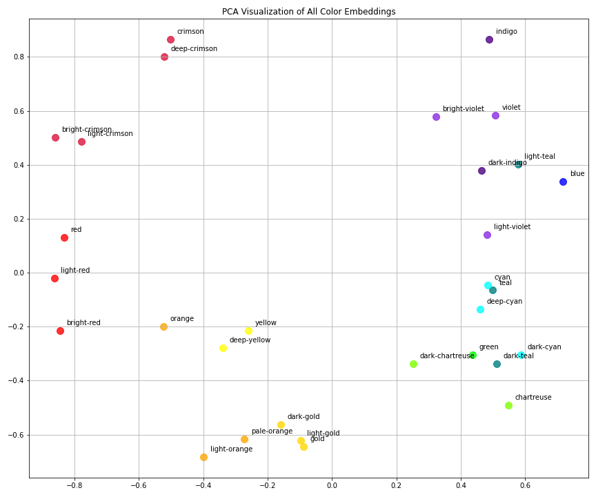
Comparing Embedding Results from Different Hyperparameters

Configurations

Plot	Embedding Dim	Epochs	Learning Rate	Filename
1	10	1000	0.01	embedding_dim_10_num_epochs_1000_learning_rate_0.01
2	15	2000	0.05	embedding_dim_15_num_epochs_2000_learning_rate_0.05

---

The model seems to be working. In both visualizations:

• Semantically related colors (like different shades of red or yellow) are clustered together.
• Opposing color categories (e.g., reds vs. blues vs. greens) are well-separated.
• The cosine-based similarity structure is preserved — close vectors = high similarity.

---

Which Model Performed Better?

Plot 1: dim=10, epochs=1000, lr=0.01

• Pros:
• Clear separation between color families (reds, yellows, blues, etc.)
• Groups like crimson-related words and cyan-related words are tight and meaningful
• Cons:
• Some clusters (e.g., yellow/orange/gold) appear stretched or less compact
• A bit more scattered in some directions

---

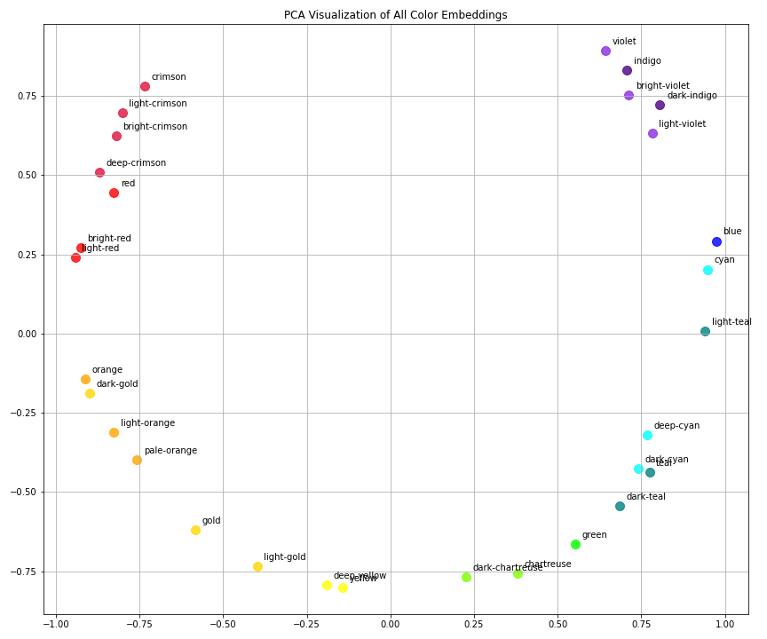
Plot 2: dim=15, epochs=2000, lr=0.05

• Pros:
• Much tighter intra-cluster cohesion, especially for:
  • Reds (crimson shades)
  • Oranges/yellows
  • Teals/cyans
• Smoother gradient flow along color transitions (e.g., from blue to green)
• Cons:
• Slightly more curvature overall (potential dimensional distortion), but not critical

---

Best Result: Plot 2

The second configuration (embedding_dim=15, num_epochs=2000, learning_rate=0.05) produced more compact and meaningful embeddings with smoother transitions and stronger separation between color categories.

Higher embedding dimension and longer training allowed the model to:

• Capture more nuance
• Better fit the similarity structure
• Learn more stable representations

---

Final Thoughts

• The model is behaving as intended.
• Hyperparameter tuning had a clear positive effect.
• We could continue experimenting with:
• Higher dims (if more color complexity exists)
• Regularization to prevent potential overfitting
• t-SNE or UMAP to visualize in 2D with less linear projection distortion

To explore the full implementation of ValueVec, including example scripts, training utilities, and both manual and neural network-based models, you can visit the official GitHub repository: github.com/rdoku/valuevec. The package is also available on PyPI for easy installation via pip: pypi.org/project/valuevec/0.1.0. Whether you're experimenting with semantic similarity using continuous labels or integrating value-based embeddings into downstream applications, ValueVec provides a flexible, open-source foundation designed for practical experimentation and research.