Neural Networks Demystified: Transformations Through Embedding Spaces

2025

Python PyTorch

Understanding Neural Networks Through Embedding Spaces

The goal of deep learning is to learn the weights and biases that activate the right neurons for the right inputs.

More specifically:

A neural network aims to learn weights and biases that:
- Activate specific pattern detectors when the relevant patterns are present in the input
- Keep those pattern detectors inactive (often using ReLU to zero out activations) when the patterns are absent
This selective activation enables the network to:
- Map similar inputs to similar regions in an embedding space
- Create decision boundaries that separate different classes of inputs
- Transform raw input data into increasingly abstract and task-relevant representations
Across layers of these learned pattern detectors:
- Early layers detect simple patterns (e.g., edges, textures, colors)
- Middle layers detect more complex patterns (e.g., shapes, parts)
- Later layers capture high-level concepts (e.g., objects, scenes, relationships)

This selective activation mechanism, enabled by non-linear functions like ReLU, is central to how neural networks learn useful representations. Non-linearities allow neurons to be truly "off" when patterns are not present, enabling the network to perform complex tasks like classification or regression.

A Simpler Way to Understand Neural Networks

Neural networks can often seem like mystical “black boxes,” but there's an elegant, intuitive way to understand them:

Neural networks are a sequence of transformations between embedding spaces. Each layer maps representations from one space to another using linear combinations followed by non-linear activations.

This article explores that transformation process step by step, revealing how neural networks learn to model complex relationships in real-world data.

Why Embedding Spaces Matter

An embedding space is a high-dimensional space where each piece of data (like a sentence, image, or table row) is represented as a vector (which you can think of as a point in that space). A vector in this context is a mathematical representation of an item. It’s a list of numbers (like [0.5, -1.2, 3.7, ...]) that captures important features or patterns about the item. Each number in the vector corresponds to a specific feature learned from the data. So, the vector itself encodes important information about the original item.

Because similar items share similar features, their vector representations are also similar. As a result, they are positioned close to each other in the embedding space. This means the location of each point in the space, determined by its vector, reflects the key characteristics of the original data item.

For example:

A small black-and-white image with 28 rows and 28 columns of pixels has 784 pixels in total. If we flatten the image into a list of 784 numbers (each number showing how light or dark a pixel is), we can think of the image as a point in a 784-dimensional space, one dimension for each pixel.

A word like “king” can be turned into a vector of 300 numbers using tools like Word2Vec or GloVe. In that space, words with similar meanings, like “queen” or “prince”, end up near each other. This helps computers understand the relationships between words.

In a table with rows of data about people, for example: age, income, and education level each row is one person’s data, and each column is one feature. So if the table has 3 columns, each person is a point in a 3-dimensional space. People with similar ages, incomes, and education levels will be located near each other in this space.

The key idea is this: similar inputs lie close together, and differences correspond to distances or directions in the space.

Neural Networks and Embedding Transformation

Neural networks turn raw input data into embeddings (vectors), and then transform those embeddings through multiple layers to make them more useful for solving tasks like classification or prediction.

Converting Input into Embeddings

Before data enters a neural network, it’s first converted into a vector form , a list of numbers that captures key features of the input. This step is sometimes called embedding or feature extraction, depending on the input type:

Images:
A 28×28 grayscale image has 784 pixels. Each pixel's intensity becomes a number, so the image is represented as a vector of 784 values.
Words or Text:
Words are turned into vectors using methods like Word2Vec, GloVe, or a learned embedding layer. Words with similar meanings end up with similar vectors.
Tabular Data:
Each column (like age, income, or category) is a feature. A row in the table becomes a vector combining these values.
Categorical Values:
Categories are mapped to dense vectors using an embedding lookup table, which is more efficient than one-hot encoding.

How Neural Networks Transform Embeddings

Once the input is turned into a vector (embedding), the neural network improves it step by step by passing it through multiple layers.

At each layer, the network does two main things:

Adjusts the Numbers (Linear Transformation):
It changes the vector using math, by multiplying it with learned weights and adding a small shift (called bias). This helps the network focus on different combinations of the input's features.
Applies a Rule (Activation Function):
It then applies a simple rule (like ReLU, which turns negative numbers into zero). This helps the network handle complex patterns instead of just straight lines.

After these steps, the vector becomes a new embedding, a new version of the data that’s slightly more useful.

This process repeats in each layer. With every step, the network fine-tunes the embedding so it becomes more and more helpful for the final task, like recognizing a number in an image, understanding a sentence, or predicting a price. By the end of this transformation chain, the network has learned a sophisticated embedding of the data, one where simple decisions (like drawing a line between categories) become possible. The purpose of this article is to walk through exactly what I just outlined, but in a way that’s simple, intuitive, and easy to digest. The goal is to demystify how neural networks work by breaking down the core ideas into clear, relatable concepts, so anyone can follow along even without a deep background in math or machine learning.

A Simple Example: Predicting House Prices

Throughout this tutorial, we'll use a straightforward example to guide us. We'll learn how a neural network can be trained to predict house prices based on a few key features.

The goal is to understand how the network learns from data and transforms raw inputs into accurate predictions.

Features We'll Use

To keep things simple, we'll use just three input features:

x₁: House size (in square feet)
x₂: Number of bedrooms
x₃: Age of the house (in years)

Sample Training Data

Here’s a small dataset we’ll work with:

House	House Size (sq ft)	Bedrooms	Age (years)	Price ($K)
1	2500	4	2	1300.8
2	1800	3	25	945.9
3	1200	2	5	649.6
4	3500	5	40	1793.5
5	800	1	1	450.1

This dataset will serve as the foundation for understanding how neural networks map inputs (features) to outputs (predicted prices).

Converting Tabular Data into Vectors

Each row in the table represents one house. To use this data in a neural network, we need to turn each house's features into a vector. A vector is simply a list of numbers.

For example, the first house has:

Size: 2500
Bedrooms: 4
Age: 2

We represent this as a vector:
[2500, 4, 2]

Each house becomes a vector like this. These vectors are the inputs to the neural network. The network will learn to take in a vector like [1800, 3, 25] and predict a price as close as possible to the actual value, such as 945.9.

Layers in a Neural Network

Input Embedding Space

The process begins in the input embedding space, which is how the data is first represented numerically before any learning happens. This can include:

Pixel values for images
Word indices or embeddings for text
Numerical features for structured or tabular data

In our house price example, each house is represented as a vector of three features:

    House 1: [2500, 4, 2]
    House 2: [1800, 3, 25]
    House 3: [1200, 2, 5]
    House 4: [3500, 5, 40]
    House 5: [800, 1, 1]

Each vector contains:

House size (in square feet)
Number of bedrooms
Age of the house (in years)

These vectors are the inputs to our neural network. The targets are the house prices we want the model to predict.

Hidden Layers

A neural network is made up of different types of layers:

The input layer receives the raw feature vectors
The hidden layers sit in between and perform most of the learning
The output layer gives the final prediction, such as a house price

A hidden layer is any layer between the input and output. It is called "hidden" because its output is not directly seen. Instead, it produces internal representations that help the model make better predictions.

You can think of the network as a step-by-step process:

The input layer receives a vector like [1800, 3, 25]
Hidden layers transform this vector, learning patterns and relationships
The output layer takes the final transformed version and predicts a value like 945.9

The hidden layers are where the learning happens. They adjust and reshape the input so that by the end, the network understands which features lead to higher or lower prices.

Hidden Layers and Neurons: The Heart of Learning

A hidden layer is composed of nodes, also called neurons, each acting as a tiny decision-maker. Every neuron is like a mini feature detector, trained to respond to a specific kind of pattern in the input data.

When data flows through a neural network, it passes from layer to layer in a structured pipeline. Each layer performs two key operations:

Linear Combination: Computes a weighted sum of the previous layer’s outputs.
Non-linear Activation: Applies a non-linear function (like ReLU) to the weighted sum.

This process transforms the data into a new embedding space, highlighting features the network finds useful and suppressing irrelevant ones. In this process, each neuron in the layer acts as a dimension in this newly constructed coordinate system. The values produced by these neurons, known as activations, represent how strongly the input matches specific patterns the network has learned to detect. Inputs that activate similar neurons will appear close together in this space, while those triggering different patterns will be pushed further apart.

This transformation is not static, it is learned. During training, the network adjusts the weights and biases so that inputs from the same category or with similar outcomes are grouped together, while dissimilar inputs are separated. Useful patterns are amplified, irrelevant features are dampened, and the resulting space becomes increasingly structured and task-relevant.

In essence, every layer builds a smarter, more abstract lens through which the network views the data. Early layers detect simple patterns. Middle layers capture more complex interactions. Deeper layers organize this information to make final decisions more accurate and interpretable. By the time the data reaches the output layer, it has been transformed through a series of embeddings tailored specifically to the problem at hand be it predicting house prices, recognizing handwritten digits, or translating language.

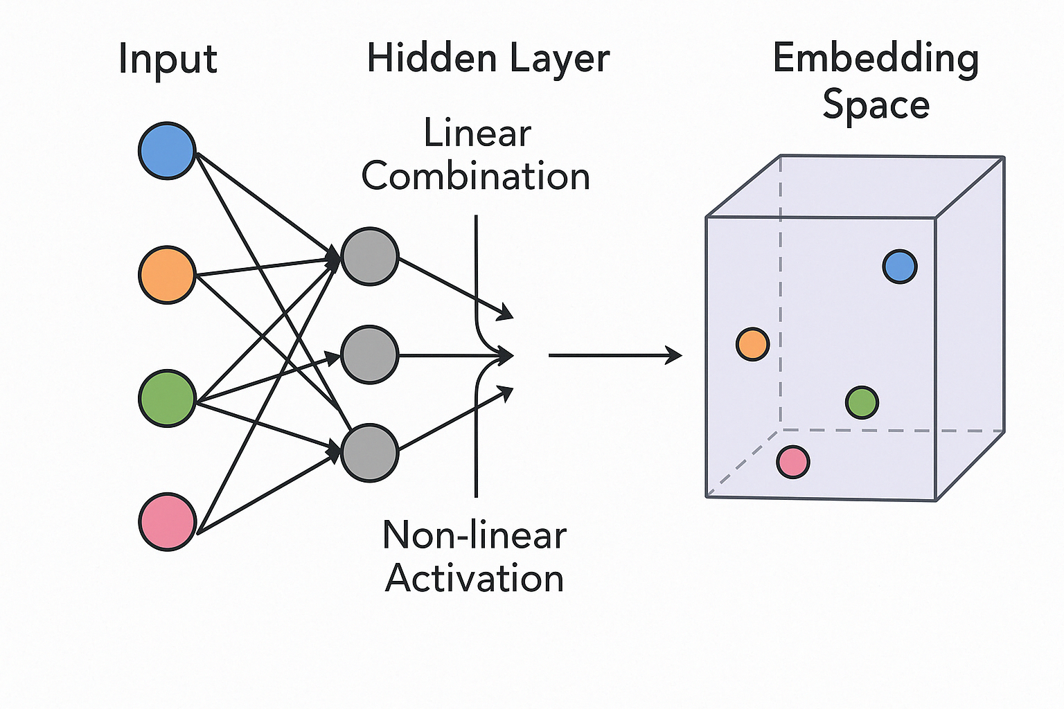
Data flowing through a neural network: Each input sample is transformed by the hidden layer into a new point in embedding space, revealing patterns the network has learned to recognize and separating inputs based on their most important features.

The image shows how house data flows through a neural network and gets transformed. On the left, four colored circles represent different houses. Each house is described by features such as size, number of bedrooms, and age. These features are combined into a vector and passed into the hidden layer.

Inside the hidden layer, each neuron processes the input by applying learned weights and adding a bias. Then it uses a non-linear function to decide how strongly it should respond to the input. If the hidden layer has three neurons, the result is a new vector with three numbers. Each number reflects how much that neuron was activated.

For example, one house might be transformed into the vector [2.0, 0.0, 1.5]. This new vector is the house’s updated representation and can be thought of as a point in a three-dimensional space.

On the right side of the image, each house is shown as a point in this new space, known as the embedding space. In this space, the neural network organizes the houses based on patterns it has learned from the data. Houses with similar characteristics appear closer together, while houses that are different are placed farther apart. This organization helps the network make more accurate predictions about prices.

Understanding the Relationship Between Inputs, Weights, and Neurons

In a fully connected (dense) layer of a neural network, each neuron is connected to every output from the previous layer. If this is the first hidden layer, those outputs come directly from the input features.

This means each neuron has:

One weight for each input feature (each number in the input vector)
One additional parameter called a bias

Formula

If you have:
I = number of input features (or the size of each input vector)
N = number of neurons in the layer

Then the total number of learnable parameters is:
(I × N) + N

The I × N part accounts for the weights
The + N adds one bias for each neuron

Then the total number of parameters (weights and biases) is:
(I × N) + N

Example

Suppose you have:
- 3 input features (such as house size, number of bedrooms, and age)
- 4 neurons in the hidden layer

Then:
- Each neuron has 3 weights and 1 bias, totaling 4 parameters
- The entire layer has 4 neurons × 4 parameters = 16 parameters

Why Does Each Neuron Need One Weight per Input?

Think of each input feature (like house size, number of bedrooms, or age) as a separate piece of information about a house.

A neuron’s job is to take all of that information and decide how important each piece is for making a prediction, such as estimating the price of a house.

To do this, the neuron assigns a weight to each input. A weight is just a number that tells the network how much to pay attention to that feature. If the weight is large, the feature has more influence. If the weight is small, the feature has less influence.

Once all the inputs are weighted, the neuron adds them together and includes a small adjustment called a bias. The total is then passed through a function to produce the neuron’s output.

In simple terms, the neuron takes all the features, uses the weights to decide what matters, and combines everything into a single number that reflects its reaction to the input.

Why One Weight per Input?

Because the neuron needs to consider every feature in the input vector, it must assign one weight to each feature. This allows the neuron to scan all the inputs and form a meaningful response.

That is why each neuron has:

One weight for every input feature
One additional bias to adjust the final result

How Many Neurons or Weights Should You Use?

The number of weights per neuron is determined by the number of input features (also called the size of the input vector). So if your input has 3 features (like [size, bedrooms, age]), each neuron needs 3 weights, one for each feature.

The number of neurons you choose in a layer is not fixed by the data. It’s a design choice you make when building the neural network. You can think of neurons as feature detectors.

If you use too few neurons, the model might miss important patterns in the data.
If you use too many neurons, the model might memorize the training data and not generalize well to new data.

A good starting point is to choose a number of neurons between the input size and the output size. It’s often best to experiment with different sizes and check how the model performs on validation or test data. Choosing the right number of neurons helps the model balance learning power with the ability to generalize to new data

Understanding Linear Combinations

As we mentioned earlier, the output of each neuron is a single number. This number is determined by a linear combination of the inputs. A linear combination, also called a weighted sum, is one of the core operations in neural networks. It multiplies each input/feature by a corresponding weight and adds them together.

Basic Formula

Given inputs:
$$ \mathbf{x} = (x_1, x_2, ..., x_n) $$

And weights:
$$ \mathbf{w} = (w_1, w_2, ..., w_n) $$

The linear combination is calculated as:
$$ z = w_1x_1 + w_2x_2 + \cdots + w_nx_n + b $$

Where:
$ z $ is the result before activation
$ b $ is the bias term

What the Weighted Sum Represents

The linear combination captures several important ideas:

Importance: The weights determine how much each input contributes to the result
Pattern Detection: The sum tells us how much the current input matches the pattern the neuron is looking for
Projection: Mathematically, it projects the input onto the direction defined by the weights
Similarity: A larger value means a stronger match between the input and the neuron's preferred pattern

How Pattern Detection Works in a Neuron

What Is Projection?

In a neural network, both the input and the weights of a neuron can be thought of as vectors — arrows pointing in space. When we compute the dot product between them (which is the linear combination), we are measuring how much the input points in the same direction as the weights.

This is called a projection. It tells us how strongly the input aligns with the pattern (weights) that the neuron has learned to recognize. A large projection means a strong match. A small or negative projection means a weak or opposite match.

Why Projection Matters

Projection is important because it gives the neuron a sense of similarity. If the input matches the pattern defined by the weights, the projection will be large, and the neuron will likely activate. This is the core idea behind pattern detection in neural networks.

But Projection Is Not Enough

Pattern detection depends on more than just projection. Several other factors play a role:

1. The Bias Term
The bias shifts the projection value up or down. This helps the neuron control when it should activate. Without a bias, the neuron would only activate when the projection is above zero. The bias adds flexibility and allows neurons to detect patterns even when inputs are small or near zero.

2. The Activation Function
After the projection and bias are calculated, the result is passed through an activation function like ReLU or sigmoid. This step decides whether the neuron should "fire" and how much of the signal should be passed forward. It introduces non-linearity, which helps the network learn more complex patterns.

3. The Input Values Themselves
The quality and scale of the input also matter. Even if the weights are well-trained, poor input values can lead to weak activations. Preprocessing, normalization, and good feature selection help ensure the network sees useful inputs.

4. The Network Context
Neurons rarely act alone. The strength of a pattern is also influenced by the combination of activations from many neurons across layers. Higher layers may recognize more abstract or combined patterns based on how lower layers respond.

Putting It All Together

Pattern detection in a neuron is driven by the projection of the input onto the weights. But to truly recognize a pattern, the network also uses the bias to shift the signal, the activation function to shape the response, and the overall architecture to combine information from multiple neurons.

The neuron is not just asking “How much does this input align with my weights?”
It is also asking “Should I respond to this pattern now, and how much should I respond?”

This layered process is what gives neural networks their power to detect and learn patterns in complex data.

Understanding the Result of a Neuron's Computation

When an input vector is passed into a neuron, the neuron computes a weighted sum by multiplying each input by its corresponding weight and adding them up. This gives a single number, often called z, which is then passed into an activation function.

But what does this number actually mean?

Interpreting the Weighted Sum

A high positive value means the input strongly aligns with the pattern the neuron has learned (i.e., the direction of the weights)
A value close to zero means the input is mostly neutral or orthogonal to the pattern — the neuron does not find anything meaningful
A negative value means the input goes against the pattern the neuron is trained to detect

This value is significant because it represents how much the input matches the neuron’s preferred pattern — which is defined by its weights.

What Is the Pattern?

The pattern a neuron is detecting is described by its weights. You can think of the weights as a kind of "template" or "filter." During training, the neuron adjusts these weights to become more sensitive to useful patterns in the input.

So, when we say the input "matches the pattern," we are really saying:

The input points in a similar direction to the weight vector in multi-dimensional space.

This similarity is measured by their dot product, also known as a projection.

Example: How a Neuron Computes the Weighted Sum

Suppose we have a neuron with the following weights:

$$ \mathbf{w} = [0.8, -0.5, 0.3] $$

And an input vector:

$$ \mathbf{x} = [0.7, 0.2, 0.9] $$

We compute the weighted sum:

$$ z = (0.8 \times 0.7) + (-0.5 \times 0.2) + (0.3 \times 0.9) = 0.56 - 0.1 + 0.27 = 0.73 $$

This value, $ z = 0.73 $, tells us how much this particular input matches the neuron's pattern.

What This Tells Us

The neuron is moderately activated by this input, since 0.73 is positive and not too small
The first feature (0.7) contributes the most positively due to the high weight of 0.8
The second feature contributes negatively, but weakly, due to both a small input (0.2) and a negative weight
The third feature (0.9) adds a moderate positive influence

This does not mean feature one is always the most important. It just means that for this specific input, it had the most impact because of its value and weight.

High Activation Example

To see what leads to stronger activation, let’s look at an input that better matches the neuron's weight pattern:

New input:

$$ x_1 = 1.0,\quad x_2 = 0.0,\quad x_3 = 1.0 $$

Weighted sum:

$$ z = (0.8 \times 1.0) + (-0.5 \times 0.0) + (0.3 \times 1.0) = 0.8 + 0 + 0.3 = 1.1 $$

This result is higher than 0.73, which means this input is a closer match to the neuron’s pattern.

Now let’s try an even stronger match:

$$ x_1 = 2.0,\quad x_2 = -1.0,\quad x_3 = 2.0 $$

Weighted sum:

$$ z = (0.8 \times 2.0) + (-0.5 \times -1.0) + (0.3 \times 2.0) = 1.6 + 0.5 + 0.6 = 2.7 $$

Here, all three input values align perfectly with the weights. The result is a very high activation of 2.7.

Key Insight

A neuron becomes highly activated when:

The input values are large where the weights are large and positive
The input values are small or negative where the weights are negative
The overall direction of the input vector is similar to the direction of the weight vector

In other words, the input is projecting strongly onto the weight vector.

The better the alignment between the input and the weights, the higher the neuron's pre-activation output. This forms the basis for pattern recognition in neural networks.

Why This Matters

This result is used in many ways within a neural network:

In classification, it helps decide which class the input belongs to
In regression, it helps determine the output value
In hidden layers, it creates new representations that are passed forward and further refined by the next layer
Every activation value contributes to a network that learns, layer by layer, how to detect useful patterns from raw data.

The Role of the Bias Term

So far, we have focused on the weighted sum of inputs and weights. But each neuron also includes a bias term, typically written as $ b $. The full equation becomes: $$ z = (w1 * x1) + (w2 * x2) + (w3 * x3) + b $$

The bias allows the neuron to shift the output value up or down. This gives the neuron flexibility to activate even when the input is small, or to stay inactive when the weighted input is large but not meaningful.

Why Bias Is Useful

Without a bias term, the neuron would always activate only when the weighted sum is above zero. This severely limits what the neuron can learn.

The bias helps in several key ways:

1. Adjusting for Smaller Input Values
When input values are small (for example, normalized to a range like [0.1, 0.05, 0.2]), even meaningful patterns may produce very small weighted sums. Without a bias, the neuron might never activate. The bias shifts the output so that the neuron can respond even when the input magnitudes are low.

2. Shifting the Activation Threshold
The bias effectively controls when a neuron decides to activate. A positive bias makes it easier to activate (lower threshold), while a negative bias makes it harder (higher threshold).

3. Increasing Learning Flexibility
The bias gives the model more freedom to fit the data, especially in situations where patterns are subtle or baseline outputs matter (such as a prediction starting from a non-zero base).

Example With Bias

Recall our earlier example where the weighted sum was:

$$ z = 0.73 $$

Now let’s see how this changes when we add a bias.

With a positive bias $ b = 0.5 $:
$$ z = 0.73 + 0.5 = 1.23 $$

With a negative bias $ b = -0.8 $:
$$ z = 0.73 - 0.8 = -0.07 $$

A positive bias makes the neuron more likely to activate, while a negative bias pushes the output downward and may suppress activation.

This is especially important when using activation functions like ReLU, which outputs zero for all negative inputs. The bias helps control when and how often a neuron activates, even when the inputs themselves are weak or limited in range.

The bias term may seem small, but it plays a big role in neural networks by:

Helping the neuron activate on small or subtle inputs
Giving the model flexibility to shift its internal thresholds
Improving the network’s ability to learn patterns and make accurate predictions

Pattern Detection in Neural Networks

What a Pattern Detector Does

When we say that a neuron acts as a pattern detector, we mean it’s learned to recognize specific combinations of input values that are meaningful for a given task. Here’s how this works:

Feature Recognition
Each neuron learns to respond strongly to certain input patterns. These patterns represent features in the data that are important for solving the task — like recognizing edges in images, or detecting relationships in tabular data.
Signal Integration
The neuron takes multiple input values (features), multiplies each by a corresponding weight, and adds them together along with a bias.
This operation (a linear combination) collapses the entire input vector into a single number. This number measures how well the input aligns with the pattern the neuron has learned to recognize.
Creating a New Representation
The output from the neuron (after applying the activation function) becomes a single value in a new vector, a new embedding.
If you have many neurons in a layer, each one outputs a value based on a different pattern. Together, these values form a new vector, which is a transformed version of the original input.
Why This Matters
This process allows the network to re-map raw input data into a new space where the relationships between inputs become more meaningful for the task.
Similar inputs (that trigger similar neurons) are placed closer together
Dissimilar inputs (that activate different neurons) are placed farther apart.
Distributed Representation
Each neuron contributes one value to the new embedding, and different neurons learn to specialize in different aspects of the input. This creates a rich, distributed representation of the data, where no single neuron captures everything — but together they describe the input from many useful perspectives.

In effect, the network is building a custom coordinate system where it becomes easier to separate, group, or classify inputs based on their underlying patterns. Neurons act as pattern detectors by computing a weighted sum of input features. This sum becomes a single output that represents how strongly the input matches the neuron's pattern.
These outputs become dimensions in a new vector space (an embedding space) that makes it easier for the network to learn, compare, and make predictions about data.

Simple Example

Imagine a neuron in a housing price prediction network with weights: [0.8, -0.5, 0.3]

This neuron is connected to three input features:

$ x_1 $: House size (in square feet)
$ x_2 $: Number of bedrooms
$ x_3 $: Age of the house (in years)

Here’s what happens:

If the house is large, has fewer bedrooms, and is relatively new, this matches the neuron's pattern:
The weighted sum will be large and positive.
The neuron becomes activated, indicating a strong match to the pattern it was trained to detect — such as a high-value home.
If the pattern is the opposite — a small, old house with many bedrooms:
The weighted sum may become small or negative.
The neuron’s activation is low or suppressed, signaling a mismatch with the pattern it responds to.

This simple example shows how a neuron identifies patterns in input features. Each neuron acts as a filter, responding only when the combination of inputs aligns with its learned weights. Its output becomes part of a new vector representation used by the next layer in the network.

Real-World Examples of Pattern Detection

Pattern detectors emerge naturally during training and vary based on the domain:

Image recognition

Early layers: detect edges, corners, textures Later layers: detect complex shapes like faces, wheels, or objects
Language models

Detect grammatical structures, topics, emotions, or tone
Audio processing

Detect frequencies, pitch patterns, or speech components

Neurons aren’t explicitly told what to look for, they learn through gradient-based training to focus on patterns that improve task performance.

Why Neurons Tend to Specialize

Neurons in a neural network are not explicitly told what to learn, but over time they often begin to specialize. This means different neurons respond to different types of input patterns. Several factors contribute to this natural specialization:

Redundancy is Inefficient
If two neurons respond to the same pattern, one becomes unnecessary. During training, backpropagation adjusts the network to reduce this overlap and encourage diversity.
Different Starting Points
Each neuron starts with its own randomly initialized weights. These small initial differences lead neurons to respond to different aspects of the input. As training progresses, these differences are amplified.
Learning Dynamics
When a neuron performs slightly better than others for a certain pattern, it receives stronger updates during training. This helps it improve even more at detecting that pattern, gradually "claiming" it.
Optimization Pressure
The training process aims to reduce the overall loss. The most efficient way to do this is for neurons to divide up the task, with each neuron handling different pieces of the input space.

Why Some Overlap Still Happens

Although neurons often specialize, they don’t do so perfectly. In fact, some overlap can be helpful:

Partial Sharing
Neurons may detect similar patterns with slight differences in angle, position, or scale.
Distributed Representations
Important patterns are often captured by groups of neurons working together, rather than just one.
Built-In Redundancy
Having some overlap improves the model’s robustness. If one neuron fails to activate, another may still respond.

Example of Natural Specialization

In a digit recognition task like MNIST:

One neuron might respond to loops, such as those in digits 0, 6, 8, and 9
Another might activate when it sees vertical lines, such as in digits 1, 4, or 7
A third might focus on diagonal strokes, like those in digits 2 or 7

No one programs these roles. The specialization emerges naturally from the training process.

How to Encourage Specialization

In some cases, it’s useful to guide the network to specialize more clearly. This can be done with:

Sparsity constraints, which limit how many neurons are allowed to activate at once
Dropout, which randomly deactivates neurons during training so others must take on more responsibility
Competitive mechanisms, which create pressure for neurons to compete for the right to respond to a pattern

Neural networks are powerful because they can divide up complex tasks into smaller pieces. Each neuron learns to detect certain features, and together they build rich, layered representations of the input data. This self-organized division of labor allows networks to handle everything from images and sounds to text and tabular data with surprising flexibility.

Why Non-Linearity Matters in Neural Networks

Activation functions play a central role in neural networks. They decide how much of a neuron's signal is passed forward to the next layer. The most important activation functions are non-linear, such as ReLU (Rectified Linear Unit).

ReLU and Selective Pattern Detection

ReLU is defined as:

ReLU(x) = max(0, x).

This simple function introduces a powerful behavior. It allows the network to turn off certain signals entirely. Here's what happens:

Negative signals are removed completely
If a neuron’s weighted sum is less than zero, ReLU outputs zero. The neuron is effectively silenced. It does not activate at all.
Irrelevant patterns are excluded from the representation
Each neuron’s output becomes one dimension in a new vector, also called an embedding. When ReLU returns zero, that entire dimension is removed from the representation. This is not just a small contribution. It is a complete absence. The network is saying, "This feature is not useful here."
The embedding space becomes sparse and meaningful
Since many neurons may output zero for a given input, the resulting vector focuses only on the features that matter most. This makes the embedding more efficient and easier for the next layer to work with.
The network learns to focus only on useful information
ReLU allows the model to be selective. Only neurons that detect helpful patterns activate and contribute to the embedding. Neurons that do not find a match remain silent.

This selective behavior shapes the embedding space. Each active neuron becomes one dimension in that space, representing a meaningful aspect of the input. When ReLU outputs zero, it tells the network to ignore that feature completely for this input.

Over time, the network learns to represent data in a compact and structured way, where each dimension highlights something useful, and unimportant signals are filtered out automatically.

What Happens with Only Linear Activations?

If we used only a linear function such as $ f(x) = x $, the network would lose this ability. Everything would be passed through, no matter how irrelevant.

Every pattern is allowed through the network
Whether a neuron’s output is helpful or not, it is included in the next layer.
Negative signals are treated the same as positive ones
There is no way to turn a neuron off. Even weak or harmful patterns still affect the result.
The network cannot perform true feature selection
Every input influences the final output, even if it is unimportant or misleading.

Why Non-Linearity Is Essential

Non-linear activation functions, such as ReLU, are not just helpful. They are required for neural networks to work well on real-world problems. Without them, a neural network would be extremely limited in what it could learn or represent.

Without non-linearity, multiple layers collapse into one

If you build a network with only linear activation functions, even if you stack many layers, the entire network behaves like just one layer. This is because the combination of linear transformations is still just another linear transformation. You could replace the whole network with a single matrix multiplication.

In other words, a deep network without non-linearity is just a larger version of a linear regression model. It may look more complex, but mathematically, it can only learn straight-line relationships. Adding more layers does not add more power unless you include non-linear activation functions between them.

The model cannot handle complex patterns in real data

Most real-world problems are non-linear by nature. For example, the price of a house might increase with size but decrease with age. A student’s grade may depend on a combination of study time and sleep, not just one factor. These relationships are curved, conditional, and sometimes involve thresholds.

A network that only uses linear functions cannot model this kind of complexity. It can only fit flat lines or planes, which often fail to capture the true structure in the data.

The network cannot detect meaningful feature combinations

Linear models cannot make decisions based on combinations or comparisons. They cannot capture logic such as “either feature A or feature B, but not both.” For example, they cannot solve the XOR problem, which requires non-linear separation.

Without non-linearity, the network loses the ability to form meaningful internal representations. It cannot build high-level features from low-level ones. It simply mixes the input features with different weights, without transforming them in useful ways.

Embedding Space Without Non-Linearity

When neurons do not use non-linear activation functions like ReLU, every neuron always outputs some value, even for irrelevant patterns. That means every dimension in the new embedding is always active.

There are no zeros, no silencing of unimportant signals. Every input contributes to every new feature. This leads to a dense embedding, where noise and unhelpful features are preserved and passed forward.

In contrast, non-linearity (especially ReLU) introduces sparsity. If a pattern is not useful, the neuron outputs zero. That feature is turned off. The embedding becomes sparse and focused, containing only the dimensions that matter for that specific input.

This is important because it makes the next layer’s job easier. It does not need to sort through unnecessary information. It only receives features that the previous layer found relevant.

Non-linearity allows a neural network to learn more than just weighted averages. It enables the network to detect patterns, filter out noise, and build deeper, more abstract representations. Without it, the network cannot model the complexity of the real world and becomes little more than a layered linear model with no real power.

Discrete Pattern Selection via ReLU

Non-linear activation functions like ReLU do more than introduce flexibility into the model. They also allow the network to make clear yes-or-no decisions about which patterns to keep.

ReLU provides a simple but powerful form of binary pattern selection:

If a neuron detects a meaningful pattern, the weighted sum is positive, and ReLU passes that value forward.
If the pattern is weak or irrelevant, the weighted sum is negative, and ReLU returns zero. That neuron is effectively silenced.

This means each neuron acts as a gatekeeper, deciding whether its feature should be included in the next layer’s representation.

For example, imagine a neuron detects "thickness" in an image. If that feature helps classify the object, the neuron activates and contributes to the embedding. But if thickness is irrelevant for the current input, the neuron outputs zero. That feature is completely ignored by all future layers.

This behavior is only possible because of non-linearity. A linear function cannot discard a feature entirely—it can only shrink it. ReLU allows the network to prune features entirely, creating clean, focused embeddings tailored to the specific input.

This selective filtering supports sparsity, improves efficiency, and helps the network build structured internal representations. It ensures that each embedding contains only the patterns that matter.

Without non-linear activation functions, neural networks would be limited to modeling simple, linear relationships. This significantly restricts their ability to solve complex tasks, such as image recognition, natural language processing, or even predicting real estate prices.

Why Non-Linearity Is Essential

What Is a Linear Relationship?

A linear relationship means the output is calculated as a weighted sum of the inputs, plus a bias:

$$ \text{Output} = w_1x_1 + w_2x_2 + w_3x_3 + \dots + b $$

This is the same idea behind linear regression.

Concrete Example: Predicting House Prices

Suppose we want to predict the price of a house based on three features:

$ x_1 $: House size in square feet
$ x_2 $: Number of bedrooms
$ x_3 $: Age of the house in years

A linear model might express the relationship as:

$$ \text{Price} = 100x_1 + 5000x_2 - 500x_3 + 50000 $$

This equation means:

Each square foot adds \$100 to the price
Each bedroom adds \$5,000
Each year of age subtracts \$500
The base value of \$50,000 is a starting price that the model assumes even when all features are zero.

This base is learned during training as part of the bias term, and represents an intercept—a fixed amount that reflects what the model thinks a typical house is worth before any features are added.

Limitations of Linear Models

Linear models make some strong assumptions:

The effect of each feature is constant
The model assumes that each additional bedroom or square foot always adds the same amount to the price, no matter what the other features are.

For example, if the model says each bedroom adds \$5,000, then:

Going from 1 to 2 bedrooms adds \$5,000
Going from 3 to 4 bedrooms also adds \$5,000

This happens even if, in reality, buyers value the third or fourth bedroom less than the first few. The model does not adjust the contribution based on context.

Features do not interact
The impact of one feature does not depend on the value of another. For example, the value of an extra bedroom is assumed to be the same whether the house is large or small.
Only straight-line boundaries are possible
The model cannot create curves, thresholds, or step-like behaviors. It can only draw flat lines or planes.

This means that the decision surface the model learns is always a straight boundary. For example, if a model is trained to decide whether a house is expensive or not based on square footage and age, it might learn a rule like:

"If the house is larger than 2,000 square feet and less than 20 years old, then it's expensive."

In a linear model, this rule would be represented as a straight line separating "expensive" from "not expensive" in a 2D plot of square footage vs. age. But real-world relationships often involve curves or cutoffs.

For instance, houses might maintain value up to 30 years old, then suddenly decline. A linear model cannot draw that sudden drop or curve, it can only draw a straight dividing line, which misses the real behavior.

How ReLU Helps Model Complex Relationships

To overcome these limitations, we need non-linear activation functions. One of the most common is ReLU (Rectified Linear Unit), defined as:

$$ \text{ReLU}(x) = \max(0, x) $$

ReLU introduces non-linearity into the network, which allows it to detect and respond to more complex patterns in the data.

1. Threshold Effects

ReLU creates a clear boundary: if the input is below zero, the output is zero; if the input is above zero, the output is passed forward. This is called a hard cutoff at zero, and it allows the network to treat certain conditions like an on-off switch.

This behavior is useful when we want the network to notice when something crosses a specific threshold—like a tipping point where something changes meaningfully.

Example: House Age and Value

Let’s say we want the network to recognize that houses start to lose value quickly after 30 years.

A neuron could be trained to:

Look at the age of the house
Subtract 30 from the age
Apply ReLU to the result

This setup creates a threshold: the neuron only activates when the house is older than 30 years. Here's how it works in practice:

If a house is 25 years old, then $ \text{Age} - 30 = -5 $, and ReLU gives 0. The neuron stays silent.
If a house is 35 years old, then $ \text{Age} - 30 = 5 $, and ReLU outputs 5. The neuron activates.

This means the neuron only turns on when the house is older than 30 years, allowing the network to respond specifically to that age threshold.

It acts like a rule:

"Only start paying attention once the house becomes old enough."

How the Neuron Implements This

Let’s say the input to the network is:

$$ \mathbf{x} = [\text{size}, \text{bedrooms}, \text{age}] $$

To implement this behavior, the neuron would have:

Weights: $[0, 0, 1]$ — it ignores size and bedrooms, and focuses only on age
Bias: $-30$ — this shifts the age so that 30 becomes the activation point

The linear output before activation is:

$$ z = (0 \cdot x_1) + (0 \cdot x_2) + (1 \cdot x_3) - 30 = \text{age} - 30 $$

After applying ReLU:

$$ a = \text{ReLU}(z) = \max(0, \text{age} - 30) $$

This gives the neuron a clear cutoff at 30 years. It becomes a pattern detector for "age greater than 30," outputting how much older the house is beyond that point.

This kind of threshold-based pattern recognition is only possible with non-linear activation functions like ReLU. A purely linear model could reduce the influence of age, but it could not ignore it completely when it's below a threshold. ReLU allows the network to say, “If the house isn’t old enough, just don’t consider this feature at all.”

2. Feature Interactions Through Layer Composition

When we stack layers of neurons, each using ReLU, the network can learn combinations of features—also known as interactions. These are patterns that depend on more than one input being true at the same time. This layered approach allows the network to build increasingly abstract and meaningful concepts from simple building blocks.

Example: Housing Features and Value

Let’s walk through how this might look in a neural network that predicts house prices. The input features include:

Number of bedrooms
Region temperature (e.g., hot or cold climate)
House size
Presence of a pool

This input is first converted into a vector—a list of numbers that represent the features of one house. This vector lives in an input embedding space, where each dimension corresponds to one original feature.

Layer 1: Detecting Basic Patterns

The first layer applies weights and biases to the input vector and passes the result through ReLU. Each neuron in this layer acts as a detector for a specific feature or threshold condition.

For example:

Neuron A: Activates when the number of bedrooms is greater than 3
Neuron B: Activates when the house is located in a hot climate
Neuron C: Activates when the square footage is more than 2,000
Neuron D: Activates when a pool is present

Each of these neurons outputs a value only if its pattern is present. Otherwise, ReLU returns zero.

The outputs from all the neurons form a new vector—a transformed version of the input. This vector lives in a new embedding space, where each dimension now reflects the presence or absence of a learned pattern, not just raw input features.

Layer 2: Combining Features

This second layer takes the pattern-based embedding from Layer 1 and learns to detect combinations of those patterns.

For example:

Neuron E: Activates only when both Neuron A and Neuron B are active
This means the house has more than 3 bedrooms and is in a hot climate
Neuron F: Activates when Neuron C and Neuron D are active
This means the house is large and has a pool

The output of this layer becomes another embedding, this time reflecting more abstract features like “large home in hot climate” or “house with luxury amenities.” Each layer is essentially a coordinate transformation, creating a new vector that expresses more advanced relationships in the data.

Layer 3: Higher-Level Reasoning

Now that the network has captured these intermediate concepts, the third layer can learn even more specific combinations.

For example:

Neuron G: Activates when both Neuron E and Neuron F are active
This represents a house that is large, has a pool, is in a hot climate, and has more than 3 bedrooms

At this point, the embedding reflects very specific, high-level insights such as:

"Pools significantly increase value only when the house is large and in a hot climate."

This kind of conditional rule—which depends on multiple factors working together—is something a linear model could never express. The network has constructed it through layer-by-layer embedding transformations.

Why This Matters

Each layer in a neural network transforms the input into a new embedding space:

The first layer moves from raw features to basic patterns
The second layer embeds combinations of patterns
The third layer embeds high-level ideas, such as regional luxury preferences or buyer behavior

Because of ReLU and non-linearity, each neuron can suppress irrelevant patterns (outputting zero) and emphasize meaningful ones (positive activations). This allows the network to reshape the data step by step, embedding it into a space where useful patterns become easy to separate and predict.

These embedding transformations are what give deep neural networks their power. They don’t just pass data forward. They rewrite the data into new forms, allowing the network to build an internal understanding of what matters—and why.

3. Variable Rates of Change

In a linear model, each feature affects the output at a constant rate. That means no matter what the value is, the amount added or subtracted remains the same.

For example:

"Every bedroom adds exactly $30,000 to the house price."

This creates a straight-line relationship between number of bedrooms and price.

But in the real world, the effect of each new bedroom often changes depending on how many bedrooms the house already has. This is known as diminishing returns.

For instance:

The first bedroom might add $50,000 to the price
The second bedroom might add $30,000
Each additional bedroom beyond that might add only $10,000

This means the more you have, the less each new one is worth.

How Neural Networks Capture This

Neural networks can model this kind of behavior using ReLU and multiple neurons. Each neuron can be set up to activate only when a certain condition is met, like the number of bedrooms crossing a specific threshold.

Suppose we want the model to behave like this:

Add $50,000 for the first bedroom
Add $30,000 for the second
Add $10,000 for every bedroom beyond two

The network can use three separate neurons to represent these effects.

Neuron A: Detects at least one bedroom

Uses the input bedrooms
Applies ReLU(bedrooms - 0)
Activates for any bedroom count greater than 0
Weight is trained to output about $50,000

Neuron B: Detects at least two bedrooms

Applies ReLU(bedrooms - 1)
Activates only when bedrooms are 2 or more
Weight contributes about $30,000

Neuron C: Detects bedrooms beyond two

Applies ReLU(bedrooms - 2)
Activates only for the third bedroom and beyond
Adds $10,000 for each additional bedroom

Example Outputs

One bedroom
Neuron A activates → $50,000
Neurons B and C stay off
Two bedrooms
Neuron A and B activate → $50,000 + $30,000 = $80,000
Neuron C stays off
Four bedrooms
All three neurons activate
A and B contribute $80,000
Neuron C contributes $20,000
Total = $100,000

Why This Matters

Using ReLU and multiple neurons, the network can create a step-like pricing structure. It no longer assumes that every feature always has the same effect. Instead, it adjusts how much value a feature contributes based on its range or context.

This flexibility is important in domains like real estate, marketing, or health predictions, where features often have non-linear effects. Neural networks learn these patterns naturally, as long as they have the right architecture and non-linear activations.

4. Submodel Specialization

Neural networks can learn to assign different parts of the network to handle different types of inputs. This is made possible by the ReLU activation function, which outputs zero when a neuron does not detect its preferred pattern.

When a neuron’s output is zero, it contributes nothing to the next layer. This means that entire groups of neurons can remain inactive unless the input matches the pattern they are looking for. As a result, different groups of neurons can act like mini-experts, each specializing in specific situations.

Example: House Price Prediction Based on Age and Features

Imagine a neural network trained to predict house prices. It receives features such as:

House age
Square footage
Number of bedrooms
Pool presence
Climate zone

Now suppose the network has learned to specialize in three different scenarios.

Neuron Group A: Young Homes

This group activates when:

The house is less than 20 years old

For example:

One neuron might compute ReLU(20 - age)
When the house is 15 years old, this neuron outputs 5
When the house is 25 years old, it outputs 0

These neurons may learn patterns specific to newer homes, such as premium pricing, modern layouts, or energy efficiency.

Neuron Group B: Very Old Homes

This group activates only when the house is older than 50 years.

A neuron might compute ReLU(age - 50)
If the house is 60 years old, this neuron outputs 10
If the house is 45 years old, it outputs 0

These neurons might learn to account for depreciation, historical charm, or renovation costs.

Neuron Group C: Luxury Features in Hot Climates

This group activates when two conditions are true:

The house has a pool
The house is in a hot climate

Each condition might be detected by earlier neurons. Then:

A deeper neuron in Group C activates only when both earlier neurons are active
This means Group C only gets involved when both a pool is present and the home is in a hot climate

These neurons might learn that a pool adds more value in warmer regions where it’s used year-round.

Why This Matters

This type of conditional behavior means different parts of the network specialize based on the context of the input. You can think of each neuron group as a submodel, focusing only on a particular range or situation.

Because ReLU zeros out the output when the pattern is not matched, these submodels stay silent unless their expertise is needed. This makes the network more efficient, more flexible, and better at handling real-world data where rules and relationships often depend on specific combinations of features.

Without Non-Linearity...

Non-linear activation functions like ReLU are essential to the power of neural networks. They allow the network to model complex relationships, detect patterns conditionally, and decide which features matter for each input.

If you remove these non-linearities and use only linear activation functions, the entire structure of the network changes—and not in a good way. Here's what happens:

The Network Becomes a Single Linear Transformation

Even if you stack multiple layers in the network, each with its own weights and biases, the final result is still just one big linear equation.

Mathematically:

A linear function applied to another linear function is still linear
So, stacking 3 or 10 or even 100 linear layers is the same as having just one layer with a bigger weight matrix

This means the depth of the network adds no additional power. You are not modeling anything more complex than a straight line or flat surface.

The Model Cannot Learn Conditional Logic

In the real world, outputs often depend on specific combinations or thresholds. For example:

"Add $30,000 to the price if the house has more than 3 bedrooms"
"Decrease the value only if the house is older than 50 years and has no recent renovations"

Linear models cannot learn this kind of rule. They treat every feature as contributing a fixed amount, regardless of context.

Without non-linearity, the network cannot learn patterns like:

"Activate only if this AND that are both true"
"Ignore this feature unless another one is present"
"Change behavior once a value crosses a certain threshold"

Every Neuron Always Passes Something Forward

In a linear network, every neuron always produces a non-zero output (unless weights are exactly zero). There is no mechanism to turn off a neuron when the input doesn't match its pattern.

This means:

Irrelevant features still flow through the network
Noise and weak signals are never filtered out
Every neuron is always contributing something, even if it's meaningless

In contrast, non-linear functions like ReLU return zero when the input is not useful. This suppressive behavior is critical for keeping the network focused on the patterns that matter.

The Embeddings Become Dense and Noisy

Each layer in a neural network transforms the input into a new vector, or embedding, that captures important features.

Without non-linearity:

Every neuron in every layer produces a value
None of the values are filtered or suppressed
The resulting embeddings are dense, meaning all dimensions are filled with values

But just having values in every position is not helpful. These values:

May conflict or cancel out
May include irrelevant information
Make it harder for later layers to find meaningful patterns

You end up with embeddings that are noisy, where the signal is buried under a pile of irrelevant data.

Without non-linear activation functions:

The network loses its ability to model complexity
Every feature affects the output in a simple, fixed way
The network cannot say “this pattern matters” and “this one doesn’t”
Layer after layer just reshuffles the input without adding any real insight

In short, without non-linearity, a neural network is no better than a glorified linear regression model. What gives it intelligence is its ability to filter, suppress, combine, and activate patterns conditionally—and that all comes from non-linear activations like ReLU.

In short, non-linearity is what turns a stack of simple equations into a powerful learning system. It enables the network to go beyond linear relationships and capture the rich, complex patterns that real-world data demands.

Learning New Feature Interactions

As we have seen, one of the most powerful aspects of neural networks is their ability to create new features from raw inputs—even if those combinations were never explicitly provided.

Unlike traditional models that require hand-crafted feature combinations, neural networks learn these interactions automatically through the use of layers and non-linear activation functions like ReLU.

Revisiting the Housing Example

Suppose we start with basic input features such as:

Number of bedrooms
Region temperature
House size
Age of the house
Presence of a pool

These are the raw inputs, but the network can discover new, useful patterns by combining and transforming them.

For example, a hidden neuron might learn to detect:

"3 or more bedrooms"
"located in a hot climate"
"age less than 5 years"

These are not part of the original dataset as separate features. Instead, the network constructs them internally by applying weights, biases, and activation functions over multiple layers.

How It Works

When a hidden neuron detects a specific pattern—like a house having more than 3 bedrooms—it becomes active and outputs a positive value.

If the pattern is present, the output is a number (e.g., 4.5)
If the pattern is absent, ReLU turns the output into zero

This allows the network to include or exclude a feature from further processing based on context.

Combining Learned Patterns

In deeper layers, the network can combine several activated patterns to form more complex conditions.

For example, a later neuron might activate only if:

"3 or more bedrooms" and
"hot climate" and
"pool is present"

This neuron might learn the rule:

"Pools significantly increase value—but only when the house is large and located in a hot climate."

Such a rule is an interaction between multiple features that cannot be captured by a linear model, which treats each feature independently.

These types of relationships are common in real-world data, where the meaning of one feature often depends on others. Neural networks discover and model these interactions naturally during training.

Why Deep Networks Work

Each layer in a neural network performs a transformation, turning the input into a new embedding that captures more meaning and structure.

First layers detect simple patterns, such as thresholds or presence/absence of features
Middle layers combine patterns to form feature interactions
Final layers make decisions or predictions based on high-level concepts

This step-by-step process allows the network to move from raw numbers to a structured understanding of the problem, similar to how a person might build intuition by combining smaller ideas into larger ones.

None of this would be possible without non-linear activation functions like ReLU. They are what allow the network to:

Selectively pass forward only useful information
Build complex, layered features
Handle real-world variation and logic

Together, non-linearity and depth turn neural networks into powerful tools for learning from data.

The Final Layer: Scaling and Prediction

After passing through all the hidden layers, the data reaches the final layer of the neural network. This is typically a single neuron that produces the output prediction. In a house price prediction model, this output is a single number representing the estimated price of the house.

How the Final Output is Computed

The final layer takes the output vector from the last hidden layer and applies a linear combination:

$$ \text{Output} = w_1 \cdot h_1 + w_2 \cdot h_2 + \cdots + w_n \cdot h_n + b $$

Where:

$ h_1, h_2, \ldots, h_n $ are the outputs from the final hidden layer
$ w_1, w_2, \ldots, w_n $ are the learned weights for the output layer
$ b $ is the output bias term

This computed value becomes the predicted output, such as the house price.

Scaling to Match the Target

During training, the network learns how to scale this output to match the range of target values. If house prices in the dataset range from $100,000 to $1,000,000, the weights and bias in the final layer must be adjusted so that the predictions also fall within this range.

This scaling happens naturally during training. The process begins with random weights and poor predictions. The network compares each prediction to the actual value using a loss function, and then updates the weights and bias through backpropagation and gradient descent. Over time, the output layer learns how to scale the final linear combination to produce values that align with the training targets.

The Role of the Final Hidden Layer

The final hidden layer captures the essential features or patterns present in the input data. Its output is a vector that represents the input in a more abstract and useful form. This vector is often referred to as an embedding.

For example, a house with the following features:

2500 square feet
4 bedrooms
2 years old

might be transformed into a learned vector like:

$$ [3.2, 0.0, 5.1] $$

This vector is then passed to the output layer to compute the final prediction.

Similar Inputs Produce Similar Vectors

One of the key behaviors of neural networks is that similar inputs tend to produce similar output vectors in the hidden layers. If two houses have nearly identical features, their embeddings from the final hidden layer will be close in value. These similar vectors will lead to similar final predictions, since they are processed by the same output weights and bias.

This behavior shows that the network is learning to group similar examples in a meaningful way. It organizes the input space so that related data points are positioned close together in the learned embedding space. This structure is not hardcoded—it emerges automatically during training as the network learns how to reduce prediction errors.

As a result, the final layer serves not only as a prediction mechanism but also as a bridge between abstract representations and real-world outputs. It converts meaningful internal vectors into appropriately scaled predictions, making the network capable of generalizing to new data.

The Neural Network Training Process

Training a neural network involves teaching it to make accurate predictions by adjusting its internal parameters—weights and biases—based on its performance on known data.

Step 1: Input Data

Training begins with structured input data. In the case of house price prediction, inputs might include house size, number of bedrooms, and age of the house. Each example is turned into a vector and passed into the input layer of the network.

Step 2: Forward Pass

The data flows through the network one layer at a time. At each layer, neurons compute a weighted sum of their inputs and apply an activation function such as ReLU. These outputs then serve as inputs to the next layer.

Eventually, the data reaches the final layer, which produces a prediction—for example, the estimated house price.

Step 3: Loss Calculation

The predicted output is compared to the true value from the training data. The difference between the predicted and actual values is passed into a loss function, such as Mean Squared Error, which calculates a single value representing how wrong the prediction was.

Step 4: Backpropagation

The network then works backward, determining how much each weight contributed to the prediction error. This process, called backpropagation, uses calculus to compute how changes in each weight would affect the loss.

Step 5: Gradient Descent

Once the gradients (slopes) are known, the network updates each weight in the direction that reduces the loss. This is done using an optimization algorithm called gradient descent. The weights and biases are nudged slightly so that the next prediction will be a little more accurate.

Step 6: Repeat Over Many Examples

This process is repeated for many training examples and often across multiple passes through the entire dataset (called epochs). Each pass helps the network refine its understanding and improve its performance.

Outcome

By the end of training, the network has adjusted its internal parameters to produce predictions that closely match the actual values. It has learned to extract patterns from the input data and represent them in a way that leads to accurate outputs.

This learning process allows the network to generalize—meaning it can make good predictions not just on the training data, but also on new, unseen data.

Conclusion

This article provided an intuitive overview of how neural networks work. We focused on the high-level ideas that make these models powerful and flexible, such as how they learn patterns through layers, how similar inputs are mapped to similar vectors, and how the final layer produces predictions that align with real-world values.

We also explored how training works—from feeding in data, making predictions, computing error, and refining the network's parameters using backpropagation and gradient descent. While we kept the math light, the goal was to build a strong mental model of what each part of the network is doing and why.

In the next article, we’ll dive into more of the implementation details and mathematical foundations. That will include a deeper look at:

How gradient descent updates weights using derivatives
The role of the learning rate
How the chain rule powers backpropagation
Code examples to show these steps in action

If you now have a clearer picture of how neural networks "think," you're ready to understand how they are trained mathematically, and how you can build and train one from scratch.