Introduction to Machine Learning: Understanding Supervised Learning
This tutorial introduces machine learning from first principles, for people who are completely new to it. We'll build intuition with examples and pictures first, then add the math, then run real code on a real dataset. By the end you'll understand what machine learning is, how data becomes geometry, the difference between classification and regression, how linear regression learns, how to tell whether a model is any good, and how to check that it works on data it has never seen.
Linear regression is our focus because it's the foundation. The ideas you learn here (turn data into vectors, measure errors, minimize them, test on new data) show up in every model you'll meet later, including neural networks.
The tutorial is long, so it's split into parts. Use the table of contents to jump around:
- Parts 1–3 cover what machine learning is, how data becomes points in space, and the two kinds of questions supervised learning answers.
- Parts 4–7 build linear regression: the model, how to score a line, how gradient descent finds the best one, and how to measure the fit.
- Parts 8–11 make it practical: testing on new data, overfitting, multiple features, the end-to-end workflow, and a hands-on example in Python.
- Parts 12–13 cover where linear regression breaks down and where to go next.
Part 1: What Machine Learning Is
Imagine teaching a computer to recognize your handwriting, recommend the perfect playlist, or catch credit card fraud, without writing a single "if-then" rule. That's machine learning.
At its heart, machine learning is about finding patterns in data. Instead of programming every decision step by step, we give the computer examples and it learns the rules itself.
Think about Spotify. Rather than hard-coding "if someone likes rock, suggest more rock," Spotify looks at millions of listening habits and discovers subtle patterns, including ones no engineer would think to write down.
Rules written vs. rules learned
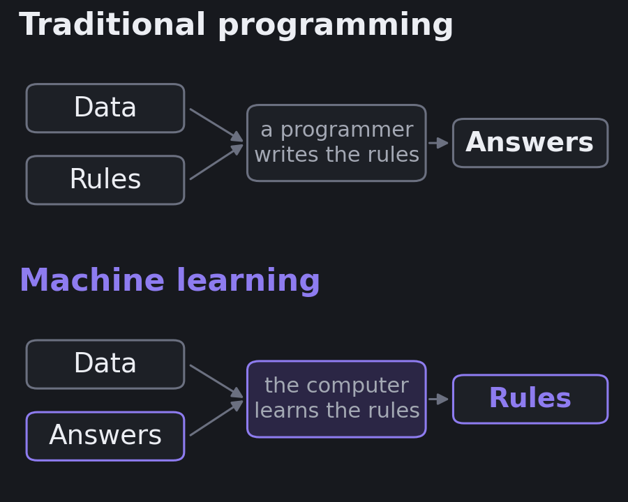
In traditional programming, a person writes the rules. You feed the program data, it applies your rules, and out come answers. A tax calculator works this way: the rules are known, so you write them down.
Machine learning flips this around. You feed in data and the answers (past examples where you know the outcome), and the computer works out the rules.
| Traditional programming | Machine learning |
|---|---|
| A person writes explicit rules | The algorithm discovers rules from examples |
| Best when the rules are clear and stable | Best when the rules are too complex to write down |
| Data + rules → answers | Data + answers → rules |
Fraud detection is a good example of why this matters. Nobody can write down every pattern that separates a fraudulent transaction from a real one, and fraudsters change tactics. A model trained on millions of labeled transactions can pick up patterns no analyst would list, and it can be retrained when the patterns shift.
Where machine learning sits inside AI
Artificial intelligence (AI) is the broad field of building machines that do things we associate with human intelligence: understanding language, recognizing images, planning, and making decisions.
Machine learning (ML) is the part of AI where systems learn from data and get better with more examples. Deep learning is a part of machine learning that uses neural networks with many layers.
Not all AI is machine learning. A chess engine that searches through possible moves, a route planner that finds the shortest path, or an "expert system" built from hand-written rules can all look intelligent without learning anything from data. Machine learning is the approach to reach for when the rules are too complex or too fuzzy to write by hand.
Three ways a machine can learn
There are three broad families:
- Supervised learning learns from labeled examples: inputs paired with the correct answer. "Here are 10,000 emails, each marked spam or not spam."
- Unsupervised learning finds structure in unlabeled data. "Here are 10,000 customers; find groups of similar ones." Nobody tells it what the groups should be.
- Reinforcement learning learns by trial and error, collecting rewards or penalties from an environment. This is how systems learn to play games or control robots.
An analogy for supervised learning: you show a child a pile of fruit and say, one at a time, "this is an apple, it goes in the apple basket; this is an orange, it goes in the orange basket." That's training, on labeled examples. Then you hand over a new pile and let the child sort it alone. That's prediction, on new data. The child is the model.
Unsupervised learning is more like being handed a messy pile of books with no categories and asked to organize them. You'd group by size, topic, or author, discovering the structure yourself.
This tutorial is about supervised learning, the most widely used of the three.
Part 2: Data as Geometry
Turning the real world into numbers
Computers understand numbers, not songs, images, or text. So we describe each real-world thing with a list of numbers called features. That list is a vector. Think of it as a digital fingerprint.
Two songs described by three features:
- Song A:
[energy: 8, danceability: 6, acoustic: 2] - Song B:
[energy: 3, danceability: 4, acoustic: 9]
Each song is now a point in 3D space. Songs that sound alike have similar vectors, so they sit close together on this invisible map. That, in a nutshell, is how a recommender can say "if you liked this, you'll like that."
Movies as vectors
Let's do the same with movies, scoring five features from 1 to 10 (these are made-up ratings for teaching, not data from anywhere):
- Action: fighting, chases, explosions
- Comedy: funny or lighthearted
- Drama: emotionally intense
- Child-friendliness: appropriate for kids
- Romance: focused on a love story
| Movie | Action | Comedy | Drama | Child-friendly | Romance | Vector |
|---|---|---|---|---|---|---|
| Avengers: Endgame | 9 | 6 | 7 | 7 | 3 | [9, 6, 7, 7, 3] |
| John Wick | 10 | 2 | 5 | 2 | 1 | [10, 2, 5, 2, 1] |
| The Lion King | 4 | 7 | 6 | 10 | 4 | [4, 7, 6, 10, 4] |
| The Notebook | 1 | 3 | 9 | 6 | 10 | [1, 3, 9, 6, 10] |
| Deadpool | 9 | 9 | 4 | 1 | 5 | [9, 9, 4, 1, 5] |
You can already see patterns. John Wick and Avengers are both high-action, but one is serious and the other funnier. The Lion King and The Notebook are both dramatic, but one is for kids and the other for adults. Deadpool is a rare mix: lots of action, lots of comedy, and not at all child-friendly.
Building up the space, one dimension at a time
Here's the key shift in thinking. You see a spreadsheet. Machine learning sees points floating in space.
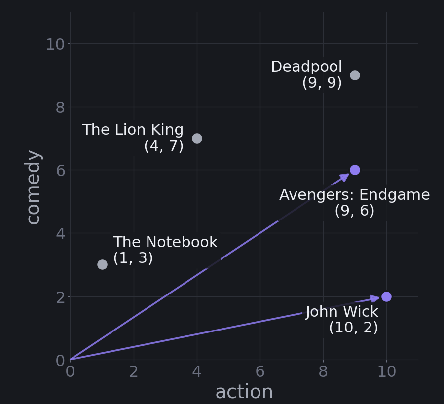
Two features. Treat each movie's numbers as coordinates, like latitude and longitude, except the axes are action and comedy. Avengers sits at (9, 6): nine for action, six for comedy. John Wick sits at (10, 2): high action, low comedy. Plot them and each movie becomes a dot on a flat map.
Three features. Add drama and each movie needs three numbers. Avengers becomes (9, 6, 7). Now the movies are points in a three-dimensional space, like the room you're sitting in, with length, width, and height.
Many features. Add romance, child-friendliness, and runtime, and each movie needs six numbers. You can't picture six dimensions. Nobody can. But the math doesn't care. Distances, directions, and lines work the same way in 6, 100, or 784 dimensions (the number of pixels in a small handwritten-digit image). Whenever you get lost, picture the 2D case and trust that the same idea carries over.
Two spaces: features in, predictions out
There are actually two separate spaces in every prediction problem:
- Feature space, where each movie lives as a point like
[9, 6, 7, 7, 3]. - Output space, where the prediction lives, such as a revenue figure or a label.
Revenue isn't inside the feature space. It's what we predict from it. Once you see data this way, machine learning becomes the job of learning a mapping from one space to the other.
Part 3: Two Kinds of Questions
Once data is in vector form, supervised learning answers two main kinds of questions.
Classification: which neighborhood?
Say we want to sort movies into Family Friendly or Not Family Friendly. We give the computer training examples that have both features and the correct label:
- The Lion King
[4, 7, 6, 10](action, comedy, drama, child-friendliness) → Family Friendly - John Wick
[10, 2, 5, 2]→ Not Family Friendly
Picture every movie as a dot in a four-dimensional space. The algorithm looks at all the labeled points and asks: where do I draw a boundary so the Family Friendly dots are on one side and the rest are on the other?
It's like dividing the space into neighborhoods. All the Family Friendly movies live in one neighborhood and the rest live in another. When a new movie arrives, the computer checks which side of the boundary its coordinates fall on.
The answer is always one of the labels. There's no middle ground.
Regression: a mathematical GPS
Now say we want to predict how much a movie will make at the box office. We give the computer each movie's features plus the actual earnings of past movies.
Box office revenue is not one of the feature dimensions. It's the target, the one number we want to predict. Regression learns a mapping that takes a movie's coordinates and tells you where it lands on the revenue scale. Think of it as a mathematical GPS: "if you're at action 9, comedy 6, drama 7, romance 3, you'll end up at this revenue."
The idea is that some features push revenue more than others. Maybe each point of action adds a certain amount, and each point of comedy adds a little less. Regression finds those amounts.
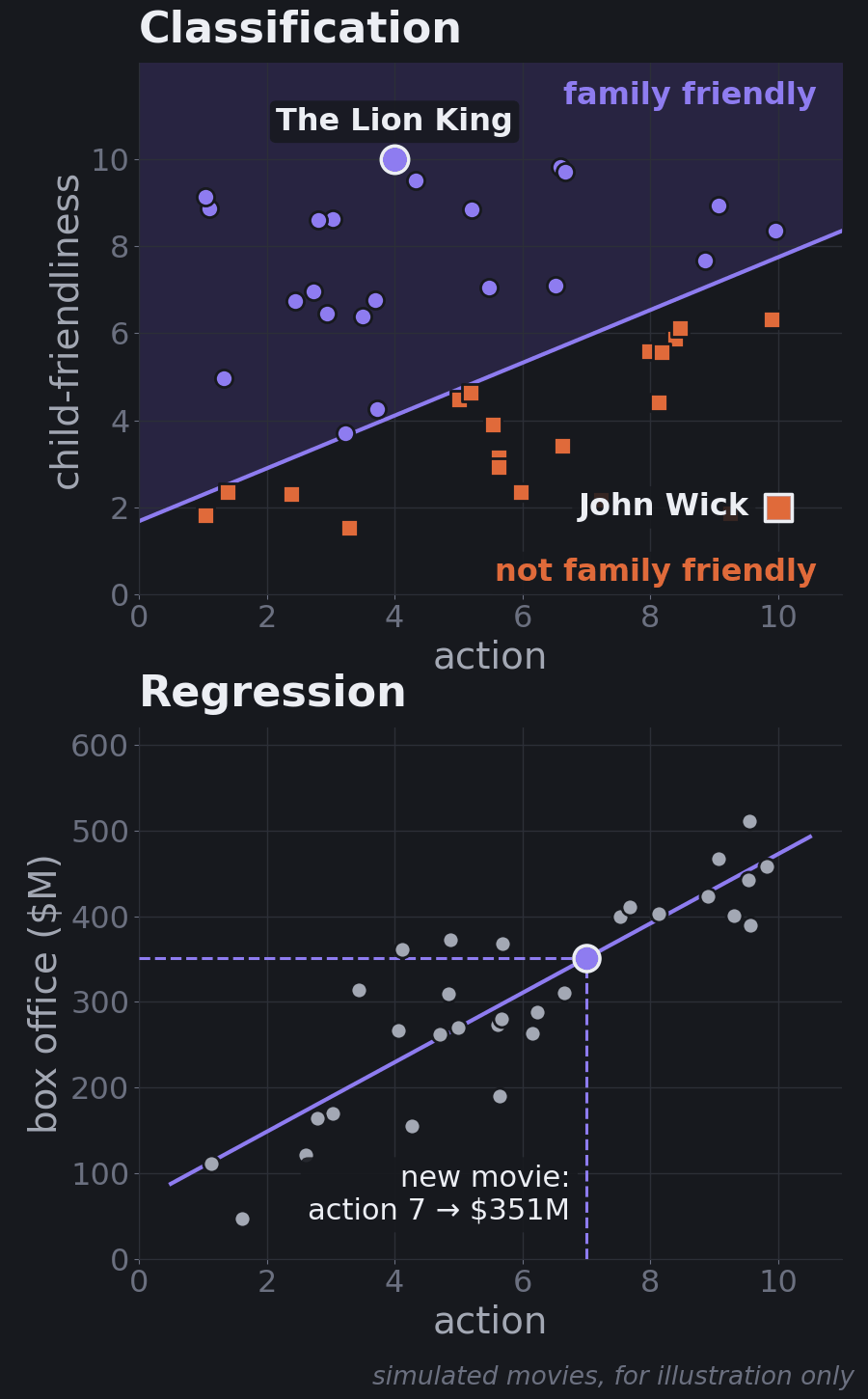
The key difference: classification learns boundaries that split the space into regions. Regression learns a mapping from many input dimensions to one target number.
Practice: which kind is it?
Try these before reading the answers.
| Question | Answer |
|---|---|
| Will this movie win an Oscar? | Classification: yes or no |
| Is this an action movie or a comedy? | Classification: one of a set of labels |
| What will this movie's IMDb rating be? | Regression: a number, like 8.5 |
| How long is this movie? | Regression: a number, like 2 hours 15 minutes |
| Which digit (0–9) is in this image? | Classification: ten labels, even though they look like numbers |
| How many cones will the stand sell tomorrow? | Regression: a count |
| Will this customer cancel next month? | Classification: yes or no |
| Will this movie earn more than $100M? | Classification: it's about money, but the answer is yes or no |
The last two rows are the useful ones. The question is never "does it involve numbers?" It's "is the answer a category or a quantity?" Digits are labels even though they're written as numbers, and "more than $100M" turns a quantity into a yes/no question.
Both are supervised learning
Classification and regression are both supervised learning, because we train on examples that include the right answer, like practicing with a teacher who shows you the answers. The model learns from those labeled examples, then predicts answers for new data that has no labels.
A simple way to remember it: classification is sorting your movie library into genre folders; regression is predicting the exact star rating you'd give each movie.
From here on, we focus on regression, and specifically on linear regression.
Part 4: Linear Regression, the Model
Why start here
Linear regression is one of the oldest and most useful models in machine learning. Banks use it to estimate risk, streaming services to estimate preferences, scientists to model climate data, and businesses to forecast sales.
It's also the "addition" you learn before "multiplication." Once it makes sense, everything else starts to make sense too. And it has a property many fancier models lack: you can read it. When it tells you each extra point of action adds a certain amount of revenue, you can see that number, question it, and decide whether to trust it.
One feature: a line
Suppose we notice that movies with more action tend to earn more. We record a few (toy numbers):
| Action level | Box office |
|---|---|
| 3 | $400M |
| 6 | $700M |
| 8 | $1.2B |
| 9 | $2.8B |
Linear regression draws the best straight line through those points. To keep the arithmetic simple, say the line comes out as:
$$\text{Revenue} = -\$500\text{M} + \$300\text{M} \times \text{Action}$$
(These are round numbers for illustration. The exact best-fit line through these four points is about −$907M + $336M × Action. You'll see how that's computed in Part 5, and why that $2.8B movie matters so much in Part 12.)
- $300M is the slope. Each extra point of action adds about $300M in revenue.
- −$500M is the intercept, where the line crosses the vertical axis. Don't worry about negative revenue. It's just the number that puts the line in the right place.
Changing these two numbers moves the line in two different ways. Changing the intercept slides the whole line up or down. Changing the slope rotates it, steeper or flatter. Every possible line is one combination of the two.
Now predict. A new superhero movie has action level 7:
$$-500\text{M} + 300\text{M} \times 7 = \$1.6\text{B}$$
That's the same \(y = mx + b\) you learned in school. Linear regression gives you three things:
- Understanding: action level really is related to revenue.
- Prediction: you can estimate earnings for a movie that hasn't come out yet.
- Strength: you can measure whether action is a strong predictor or a weak one.
The same idea predicts house prices from square footage, sales from ad spend, and grades from study hours.
Find the pattern, make predictions, minimize errors
Hold on to this three-step mantra. It describes linear regression, and it describes nearly every model you'll ever meet:
- Find the pattern (the line, or more generally the mapping).
- Make predictions with it.
- Minimize errors: adjust the pattern until the predictions are as close to reality as possible.
Linear regression just does it in the simplest way possible. Parts 5 and 6 are about step 3.
Many features: a mapping between spaces
Real predictions use many features. With all five movie features:
$$\text{Revenue} = m_1 x_1 + m_2 x_2 + m_3 x_3 + m_4 x_4 + m_5 x_5 + b$$
where \(x_1\) is action, \(x_2\) comedy, \(x_3\) drama, \(x_4\) child-friendliness, and \(x_5\) romance. Each feature gets its own weight \(m\), and \(b\) is the base amount.
This isn't really "a line" anymore; with five features it's a flat surface in six dimensions (a hyperplane). But the right way to think about it is the two spaces from Part 2: a mapping from 5D feature space to 1D output space.
That mapping is just the set of weights \(m = [m_1, \ldots, m_5]\). Suppose training on past movies taught us the weights [8, 3, 2, 5, 1] (in $M per feature point) and a base amount of $10M. To predict Avengers, multiply each feature by its weight and add them up (that's called a dot product), then add the base:
$$[9, 6, 7, 7, 3] \cdot [8, 3, 2, 5, 1] = 72 + 18 + 14 + 35 + 3 = 142$$
$$142 + 10 = \$152\text{M}$$
(These are toy numbers to show the mechanics, not real box office figures.)
import numpy as np

avengers = np.array([9, 6, 7, 7, 3])   # action, comedy, drama, child-friendly, romance
weights  = np.array([8, 3, 2, 5, 1])   # learned: $M per feature point (toy numbers)
bias     = 10                          # learned base amount, $M

predicted_revenue = avengers @ weights + bias
print(predicted_revenue)  # 152  ->  $152M
Each weight tells you how much that feature contributes. A weight of 8 on action means each extra action point adds $8M to the prediction, and a weight of 1 on romance means romance matters much less. Nobody set these weights by hand. They come from patterns in the data: if action movies consistently earned more, training automatically gives action a bigger weight.
A helpful way to picture the weights is as a lens. Feature space is what you're looking at, output space is the image, and the weights are the lens that bends one into the other. Training is the search for the right lens, the one that focuses feature vectors into accurate predictions.
Many outputs: many mappings
What if you need more than one number out? You learn more than one mapping, one weight vector per output.
- 5 → 1: movie features to revenue. One weight vector.
- 5 → 2: movie features to revenue and IMDb rating. Two weight vectors, one for each output.
- 784 → 10: the 784 pixels of a small handwritten digit image to a score for each digit 0–9. Ten weight vectors, each 784 numbers long. The digit with the highest score wins.
The last one is worth pausing on. A digit recognizer can start as nothing more than ten linear regressions sharing the same input. Neural networks stack many of these mappings with simple non-linear steps in between, which lets them bend the space in ways a single mapping can't. Neural Networks Demystified picks up exactly there.
Part 5: Which Line Is Best?
You could draw infinitely many lines through the data. How do we pick the best one? We need a way to measure how bad a line is.
Measuring error
Let's switch to a simpler example: an ice cream stand predicting cones sold from the temperature. We'll use twelve days of made-up data for teaching (not real sales), shown in the figures below.
Every prediction can be off. The gap is the error (also called the residual):
$$\text{error} = \text{actual} - \text{predicted}$$
If 50 cones were actually sold and we predicted 45, the error is +5. It's positive when we predicted too low and negative when we predicted too high. Geometrically, it's the vertical distance between a data point and the line.
Why not just add up the errors?
One day the error is +5, another day it's −5. Add them and you get 0, which looks perfect even though the model was wrong twice. Errors shouldn't cancel out.
Square them first
Instead, square each error and then add them up. This is the Sum of Squared Errors (SSE):
$$\text{SSE} = \sum_i (y_i - \hat{y}_i)^2$$
Here \(y_i\) is the actual value for day \(i\) and \(\hat{y}_i\) ("y-hat") is the prediction. +5 becomes 25, −5 also becomes 25, and the total is 50, an honest measure of how far off we were.
Squaring does three useful things:
- No cancellation. Positive and negative errors can't hide each other.
- Big mistakes count more. An error of 10 becomes 100, four times worse than an error of 5 (25).
- The math stays smooth, which makes it easy for a computer to minimize using calculus.
Now every candidate line gets a score. One small choice before we draw them: we'll measure temperature as degrees above 70°F, so the intercept means "cones sold on a 70°F day." That's easier to read than "cones sold at 0°F," and Part 9 shows it also helps the computer.
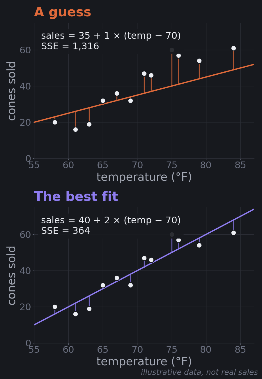
The best line is sales = 40 + 2 × (temp − 70): about 40 cones on a 70°F day, and 2 more cones for each extra degree. No other slope and intercept gets the SSE below 364.
Try it yourself
Move the sliders to change the slope and intercept and watch the residuals and the SSE change. The small map shows where your line sits on the error landscape described next. You can also let the computer take gradient-descent steps (Part 6) and compare the three learning rates.
Fit a line to the ice cream data
The error landscape
Every possible line (each combination of slope and intercept) has its own SSE. Imagine a 3D landscape: slope on one axis, intercept on another, and SSE as the height. For linear regression this landscape is shaped like a bowl. The bottom of the bowl is the line with the smallest error, the best fit.
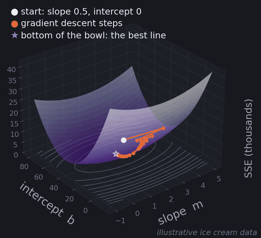
Finding that bottom is called optimization, and every machine learning algorithm does some version of it: measure how wrong you are, then make it less wrong.
For linear regression there's actually a formula that jumps straight to the bottom (the "least squares" solution, which is what np.polyfit and scikit-learn's LinearRegression use). But that shortcut only exists for this simple bowl. Most models, neural networks included, have no formula. They have to walk down. That walk is gradient descent, and it's worth understanding on the simplest landscape first.
Part 6: Gradient Descent
Walking downhill blindfolded
How does the computer get to the bottom of the bowl? It can't try every line; there are infinitely many. Instead it uses gradient descent.
Imagine being dropped blindfolded on a hillside and trying to reach the bottom of the valley. You can't see, but you can feel which way the ground slopes under your feet. So you take a small step downhill, feel again, and repeat.
- Start with a guess. For example, slope 0.5 and intercept 0. Calculate the error. You're somewhere on the side of the bowl.
- Feel the slope. The derivative (or gradient) tells you how steep the error landscape is at your position, and which way is downhill, separately for the slope and the intercept.
- Take a small step downhill. Nudge both numbers in the direction that reduces the error.
- Repeat until the ground is flat, meaning the derivatives are close to zero. You're at the bottom, and any further change would make predictions worse. This is called convergence.
Steep ground means you're far from the bottom, so the steps come out bigger. Gentle ground means you're close, so they shrink on their own.
In practice we minimize the mean squared error (MSE, the SSE divided by the number of days) rather than the SSE. It has exactly the same bottom, and the step sizes don't depend on how many data points you have. With \(e_i = y_i - (b + m x_i)\) as the error on day \(i\), the derivatives are:
$$\frac{\partial\,\text{MSE}}{\partial m} = -\frac{2}{n}\sum_i e_i\,x_i$$
$$\frac{\partial\,\text{MSE}}{\partial b} = -\frac{2}{n}\sum_i e_i$$
and each step moves against them, scaled by the learning rate \(\alpha\):
$$m \leftarrow m - \alpha\,\frac{\partial\,\text{MSE}}{\partial m}$$
$$b \leftarrow b - \alpha\,\frac{\partial\,\text{MSE}}{\partial b}$$
You don't need to derive these. Read them as: "if the errors are mostly positive (we're predicting too low), raise the intercept; if the errors are big on hot days, raise the slope."
Gradient descent in code
Here's the whole loop on the ice cream data, with nothing hidden:
import numpy as np

# Illustrative data (made up for teaching): 12 days at an ice cream stand
temp  = np.array([58, 61, 63, 65, 67, 69, 71, 72, 75, 76, 79, 84])
sales = np.array([20, 16, 19, 32, 36, 32, 47, 46, 60, 57, 54, 61])
x = temp - 70                      # degrees above 70°F

def sse(m, b):
    return np.sum((sales - (b + m * x)) ** 2)

m, b = 0.5, 0.0                    # initial guess: slope 0.5, intercept 0
lr = 0.015                         # learning rate (step size)
print(f"start     m = {m:5.2f}  b = {b:5.2f}  SSE = {sse(m, b):8.1f}")
for step in range(1, 201):
    error = sales - (b + m * x)    # actual - predicted, for every day
    dm = -2 * np.mean(error * x)   # slope of the error surface in the m direction
    db = -2 * np.mean(error)       # ... and in the b direction
    m -= lr * dm                   # step downhill
    b -= lr * db
    if step in (1, 2, 3, 10, 50, 100, 200):
        print(f"step {step:<4} m = {m:5.2f}  b = {b:5.2f}  SSE = {sse(m, b):8.1f}")

# The exact answer, for comparison (least squares solved directly)
m_best, b_best = np.polyfit(x, sales, 1)
print(f"exact     m = {m_best:5.2f}  b = {b_best:5.2f}  SSE = {sse(m_best, b_best):8.1f}")
Running it prints:
start     m =  0.50  b =  0.00  SSE =  21031.0
step 1    m =  2.94  b =  1.20  SSE =  19011.5
step 2    m =  1.40  b =  2.36  SSE =  17592.7
step 3    m =  2.38  b =  3.49  SSE =  16448.8
step 10   m =  1.99  b = 10.50  SSE =  10805.0
step 50   m =  2.00  b = 31.28  SSE =   1277.0
step 100  m =  2.00  b = 38.10  SSE =    407.4
step 200  m =  2.00  b = 39.91  SSE =    364.1
exact     m =  2.00  b = 40.00  SSE =    364.0
Read the slope column. After the first step it jumps from 0.50 to 2.94, past the right answer of 2. Then it swings back to 1.40, then 2.38, and settles at 2.00 within about ten steps. That's overshooting in action: the step was a bit too big for the slope, so it bounced across the valley before settling. The intercept moves more slowly and steadily, from 0 to 10.5 by step 10, 38.1 by step 100, and 39.91 by step 200. The SSE falls from 21,031 to 364.1, essentially the exact answer of 364.
This is how nearly every model learns: start with some parameters, measure how wrong the predictions are, work out which direction reduces the error, take a small step, and repeat. Linear regression walks a landscape with two parameters. A neural network walks one with millions. The principle is identical. It's systematic optimization, nothing more mysterious than that.
The learning rate
The size of each step is the learning rate, and choosing it is a balancing act.
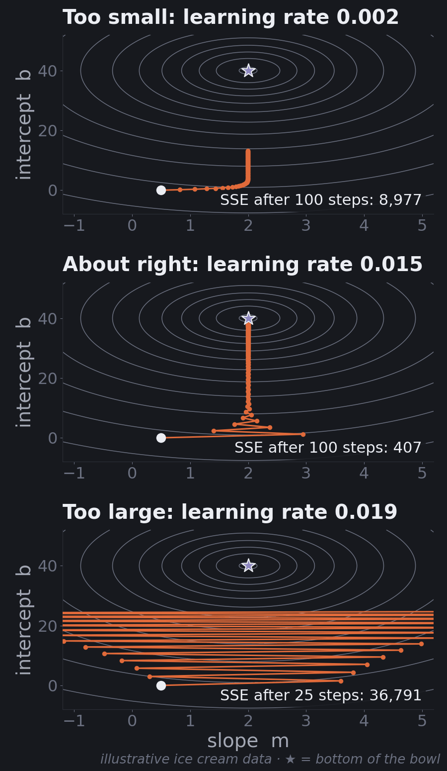
- Too small (0.002): every step is safe but tiny. After 100 steps the SSE is still 8,977, far from 364. You'd get there eventually, but it wastes time.
- About right (0.015): after 100 steps the SSE is 407, and it's within 1% of the minimum by step 141. The first few steps overshoot on the slope, then settle.
- Too large (0.019): each step overshoots by more than the last. The slope bounces from one side of the valley to the other, further each time, and after 25 steps the SSE has grown to 36,791. Keep going and it heads to infinity.
Notice how small the gap is between "about right" and "too large" here (0.015 vs. 0.019). That's typical, and it's why the learning rate is one of the first things practitioners tune. Part 9 shows a simple trick that makes the bowl rounder and widens that safe range a lot.
Part 7: How Good Is the Fit?
We have the best line. Is it any good?
Explained and unexplained
For each prediction, there are three important values:
- \(y\): the actual value.
- \(\hat{y}\): our prediction.
- \(\bar{y}\) ("y-bar"): the average of all actual values. This is what you'd guess if you knew nothing about the features.
These split each data point's story into two parts:
- Explained: \(\hat{y} - \bar{y}\). How much better our prediction is than just guessing the average.
- Unexplained: \(y - \hat{y}\). The error, the part our model can't account for.
Example. On a 75°F day, the stand actually sold 60 cones. The model predicted 50, and the average day sells 40.
- Explained: 50 − 40 = 10 cones. The model knows hot days sell more.
- Unexplained: 60 − 50 = 10 cones. Something else helped that day. Maybe it was a holiday, or there was a festival nearby. The model only knows about temperature.
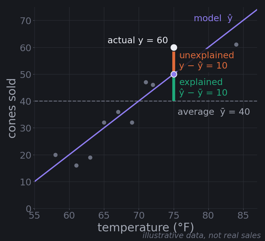
A good model makes the explained part as large as possible and the unexplained part as small as possible.
R-squared
Square those pieces and add them up across every data point:
- SST (Sum of Squares Total): \(\sum (y - \bar{y})^2\), all the variation in the data, meaning how much sales differ from the average overall.
- SSR (Sum of Squares Regression): \(\sum (\hat{y} - \bar{y})^2\), the variation the model explains.
- SSE (Sum of Squares Error): \(\sum (y - \hat{y})^2\), the variation it doesn't.
For a least-squares line with an intercept (which is what linear regression produces), SST = SSR + SSE. On our twelve days: SST is 2,972, SSE is 364, and SSR is 2,608.
R-squared is the share of the variation the model explains:
$$R^2 = 1 - \frac{\text{SSE}}{\text{SST}}$$
For a least-squares fit with an intercept, that's the same as SSR / SST. For the ice cream line it's 1 − 364 / 2,972 ≈ 0.88: temperature explains about 88% of the day-to-day variation in sales.
An \(R^2\) of 0.8 means the model explains 80% of the variation and 20% is still unexplained. An \(R^2\) of 0.3 means 70% is a mystery, so maybe you need more features, like humidity, day of the week, or local events. An \(R^2\) of 0 means the model does no better than predicting the average every time.
Because SST is fixed by the data, explaining more (higher SSR) automatically means less error (lower SSE). That's why minimizing squared error works: it's the same thing as maximizing what the model explains.
R-squared is a handy scorecard for comparing models. If adding humidity raises \(R^2\) from 0.6 to 0.8, humidity helped. But keep its limits in mind:
- On training data, it never goes down when you add features, even useless ones. A more complex model can score higher and still predict worse on new data. (Part 8 is about exactly this.)
- It says nothing about the size of the errors. A model can explain 90% of the variation and still be off by hundreds of cones on individual days.
- On new data it can be negative, if the model does worse than predicting the average. You'll see a (tiny) negative one in Part 11.
Error metrics: MSE, RMSE, MAE
These tell you how big the errors actually are, in real units:
- Mean Squared Error (MSE): the average squared error, SSE divided by the number of points. It's in "squared cones," which is hard to interpret.
- Root Mean Squared Error (RMSE): the square root of MSE, back in cones. Roughly, "a typical prediction is off by about this much."
- Mean Absolute Error (MAE): the average of the absolute errors. "A typical error is this many cones, in either direction."
A quick example: with 100 days of data and an SSE of 5,000, the MSE is 5,000 / 100 = 50 squared cones, and the RMSE is \(\sqrt{50} \approx 7.07\) cones. Now you can say "our predictions are typically off by about 7 cones."
RMSE punishes big errors more than MAE, because it squares them first. If RMSE is much bigger than MAE, your model is making a few large mistakes.
Worked example: five days of ice cream
Here's a separate, smaller example: five days of predictions from some model (made-up numbers for teaching).
| Day | Predicted | Actual | Error (actual − predicted) | Squared |
|---|---|---|---|---|
| 1 | 50 | 45 | −5 | 25 |
| 2 | 30 | 35 | +5 | 25 |
| 3 | 60 | 70 | +10 | 100 |
| 4 | 40 | 40 | 0 | 0 |
| 5 | 25 | 40 | +15 | 225 |
- MAE = (5 + 5 + 10 + 0 + 15) / 5 = 7 cones
- MSE = (25 + 25 + 100 + 0 + 225) / 5 = 75
- RMSE = √75 ≈ 8.66 cones
RMSE is higher than MAE because day 5's 15-cone miss gets heavily penalized when squared.
For R-squared: the average of the actual sales is 46 cones. SSE is 375, and SST (the squared distances of each actual value from 46) is 770. So:
$$R^2 = 1 - \frac{375}{770} \approx 0.51$$
The model explains about half the variation in sales. Here's the same calculation in code, checked against scikit-learn:
import numpy as np
from sklearn.metrics import mean_absolute_error, mean_squared_error, r2_score

predicted = np.array([50, 30, 60, 40, 25])
actual    = np.array([45, 35, 70, 40, 40])

error = actual - predicted
print("errors:", error)
print("MAE  =", np.mean(np.abs(error)))
print("MSE  =", np.mean(error ** 2))
print("RMSE =", round(np.sqrt(np.mean(error ** 2)), 2))

sse = np.sum(error ** 2)
sst = np.sum((actual - actual.mean()) ** 2)
print("mean =", actual.mean(), " SSE =", sse, " SST =", sst, " R2 =", round(1 - sse / sst, 2))

# scikit-learn agrees
print(mean_absolute_error(actual, predicted), mean_squared_error(actual, predicted),
round(r2_score(actual, predicted), 2))errors: [-5 5 10 0 15]
MAE = 7.0
MSE = 75.0
RMSE = 8.66
mean = 46.0 SSE = 375 SST = 770.0 R2 = 0.51
7.0 75.0 0.51Which metric should you use?
- R-squared to see how much of the variation the model captures, and to compare feature sets.
- RMSE when large mistakes are especially costly.
- MAE for the most intuitive "typical error," when all mistakes matter equally.
In practice, report all three. What counts as "good" depends on the problem: an RMSE of 2 cones might be excellent for an ice cream stand, while an RMSE of $50,000 might be terrible for house prices. Always compare against a sensible baseline, like predicting the average. And, most important of all, measure them on data the model didn't train on. That's the next part.
Part 8: Will It Work on New Data?
Everything so far measured how well a line fits the data it was trained on. That's not the goal. Nobody needs a model to "predict" last summer's sales; they already know them. The goal is to predict days that haven't happened yet. This is called generalization, and it's the most important idea in this tutorial after the line itself.
The true relationship
Linear regression assumes there's a true relationship in the world, some rule that really governs how temperature affects sales, plus random noise on top. We can never see that rule directly. Every dataset we collect is a sample from it, and every line we fit is an estimate of it.
Different samples give slightly different lines. To make that concrete, the figure below cheats: it invents a true rule (40 + 2 × (temp − 70), plus random day-to-day noise), draws five separate samples of twelve days from it, and fits a line to each.
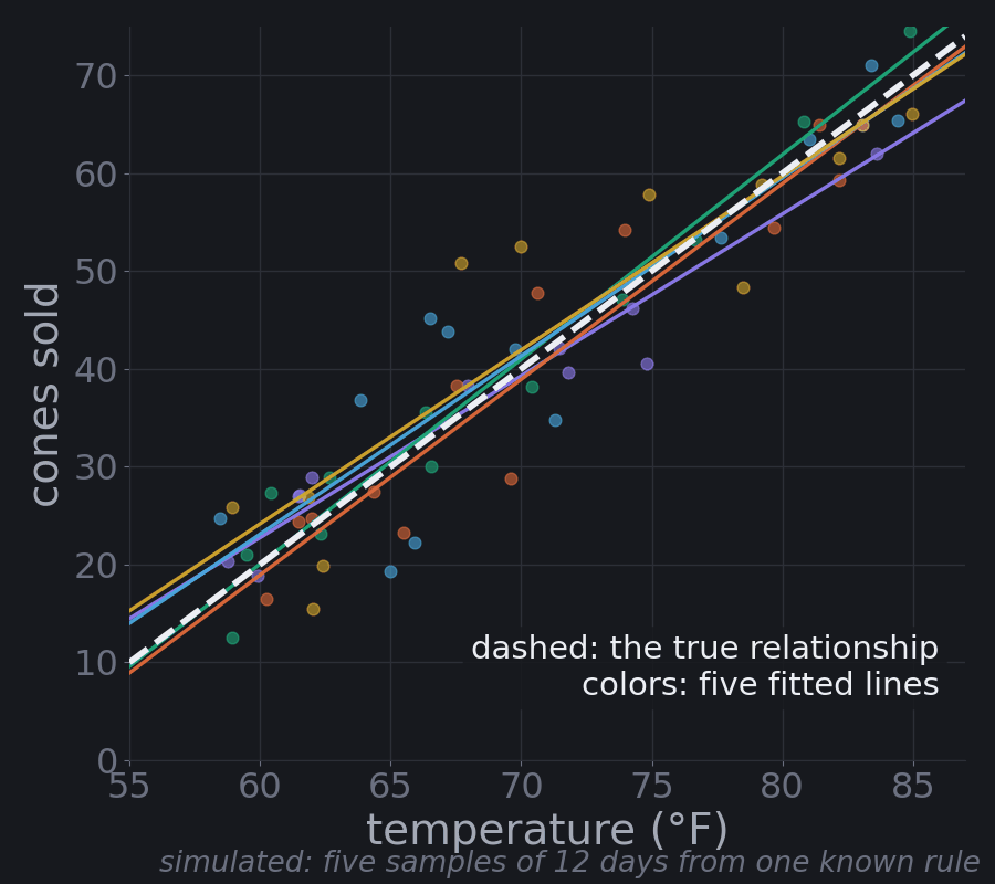
All five lines are trying to estimate the same thing, and none of them is exactly right. That's the honest picture of every model you'll ever fit: the training data is one sample, the model is shaped partly by the real pattern and partly by that sample's noise, and the question is how well it does on the next sample.
Training data and test data
The fix is simple and non-negotiable: hold some data back.
- Training set (typically 70–80% of the data): the model learns from this.
- Test set (the rest): the model never sees it during training. You use it once, at the end, to estimate how the model will do on new data.
The test set is the new pile of fruit from Part 1: the child sorted the training pile with your help, and now you see how they do alone. If you peek at the test set while building the model (choosing features by test score, say), it stops being new, and your estimate becomes too optimistic. When you need to compare many options, split off a third piece, a validation set, or use cross-validation, which rotates which slice of the training data plays "validation" and averages the results.
Underfitting and overfitting
A model can fail to generalize in two opposite ways.
Underfitting is studying only the chapter titles. The model is too simple to capture the real pattern, so it does poorly on training data and new data.
Overfitting is memorizing last year's exam answers. The model is so flexible that it learns the noise in the training data along with the pattern. It looks excellent on the training data and does poorly on anything new.
To see both, we can give linear regression curved features. A polynomial model adds columns like \(x^2\), \(x^3\), and so on, then fits an ordinary linear regression on them. The "degree" is the highest power, and a higher degree means a more flexible curve. Below, the data is simulated from a known wavy curve plus noise: 20 training points, and 500 fresh test points from the same range.
import numpy as np
from sklearn.pipeline import make_pipeline
from sklearn.preprocessing import PolynomialFeatures
from sklearn.linear_model import LinearRegression
from sklearn.metrics import mean_squared_error

# Simulated data: a known curved "true relationship" plus random noise.
# 20 training points; 500 fresh test points from the same range.
rng = np.random.default_rng(0)
def true_f(x):
    return np.sin(2 * np.pi * x)

x_train = np.sort(rng.uniform(0, 1, 20)); y_train = true_f(x_train) + rng.normal(0, 0.25, 20)
x_test  = rng.uniform(x_train.min(), x_train.max(), 500)
y_test  = true_f(x_test) + rng.normal(0, 0.25, 500)

for degree in (1, 3, 15):
    model = make_pipeline(PolynomialFeatures(degree), LinearRegression())
    model.fit(x_train[:, None], y_train)
    rmse_train = mean_squared_error(y_train, model.predict(x_train[:, None])) ** 0.5
    rmse_test  = mean_squared_error(y_test,  model.predict(x_test[:, None])) ** 0.5
print(f"degree {degree:>2}: train RMSE = {rmse_train:.2f} test RMSE = {rmse_test:.2f}")degree 1: train RMSE = 0.47 test RMSE = 0.51
degree 3: train RMSE = 0.13 test RMSE = 0.26
degree 15: train RMSE = 0.05 test RMSE = 1.23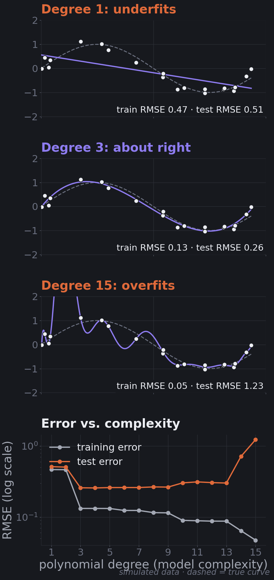
Read the numbers:
- Degree 1 underfits. Training error 0.47, test error 0.51. Both are bad, and close to each other.
- Degree 3 is about right. Training error 0.13, test error 0.26. The test error is close to the noise we added (0.25), which is about as good as any model can do.
- Degree 15 overfits. Its training error is the lowest of all, 0.05, so it looks like the best model. But its test error is 1.23, almost five times worse than degree 3.
The bottom panel of the figure is the classic picture. Training error almost always falls as you add complexity. Test error falls, then rises. The sweet spot is where test error is lowest. Two quick diagnostics follow from it:
- Both errors high → underfitting. Try a more flexible model or better features.
- Training error low, test error much higher → overfitting. Try a simpler model, more data, or regularization (a penalty on large weights that keeps the model from contorting itself; ridge and lasso regression are the linear-regression versions).
Generalization is the real score
This changes how to read Part 7. R², RMSE, and MAE on the training data tell you how well the model memorized. The same metrics on the test data tell you how well it learned. Only the second one matters for the job you're building the model to do. When someone reports a high R², your first question should be "on what data?"
Part 9: Multiple Regression in Practice
Real models have many features. Three practical ideas make them work.
"Holding everything else constant"
In a model with several features, each weight means: how much the prediction changes when this feature goes up by one unit and every other feature stays the same.
That last part matters. In the movie model, the action weight of 8 means "one more point of action, for a movie with the same comedy, drama, child-friendliness, and romance, adds $8M." It does not mean "movies with more action earn $8M more," because in real data, high-action movies may also differ in other ways (they may be less romantic, for example). Simple regression on action alone would mix those effects together. Multiple regression tries to separate them.
You'll see this happen with real numbers in Part 11: body mass index has a slope of 10.76 when it's the only feature, and 5.85 once nine other measurements are in the model. Part of what BMI seemed to explain on its own was really being carried by things that go along with it.
Categories: one-hot encoding
Regression needs numbers, but many useful features are categories: genre, city, day of the week. You can't just code genre as action = 1, comedy = 2, romance = 3. That tells the model romance is "three times" action and that comedy sits exactly halfway between them, which is nonsense.
Instead, use one-hot encoding: one 0/1 column per category.
import pandas as pd

movies = pd.DataFrame({
    "movie":  ["John Wick", "Deadpool", "The Notebook", "The Lion King"],
    "action": [10, 9, 1, 4],
    "genre":  ["action", "comedy", "romance", "animation"],
})

# One 0/1 column per genre. drop_first removes the first genre
# alphabetically ("action"), which becomes the reference genre.
encoded = pd.get_dummies(movies, columns=["genre"], drop_first=True, dtype=int)
print(encoded.to_string(index=False)) movie action genre_animation genre_comedy genre_romance
John Wick 10 0 0 0
Deadpool 9 0 1 0
The Notebook 1 0 0 1
The Lion King 4 1 0 0Each genre gets its own column, and each column gets its own weight. One genre (here "action") is dropped and becomes the reference: John Wick has zeros in every genre column, and the comedy weight means "how much more (or less) a comedy earns than an otherwise identical action movie." Dropping one column avoids redundancy: if a movie isn't comedy, romance, or animation, it must be action, so a fourth column would add no information and would confuse the fit.
Feature scaling
Features often live on wildly different scales. In Part 11, age is measured in years (19 to 79) and one blood measurement is around 3 to 6. Two problems follow.
Comparing weights. A weight is "per one unit," and units differ. A weight of 0.14 per year of age and 67 per unit of a blood measurement aren't comparable. If you standardize each feature first (subtract its mean, divide by its standard deviation), every weight becomes "per one standard deviation," and you can compare them directly.
Gradient descent. This is the less obvious one. When features are on very different scales, the error bowl gets stretched into a long, narrow valley. Gradient descent then has a terrible choice: a learning rate big enough to make progress along the valley overshoots across it, and one small enough to stay stable barely moves.
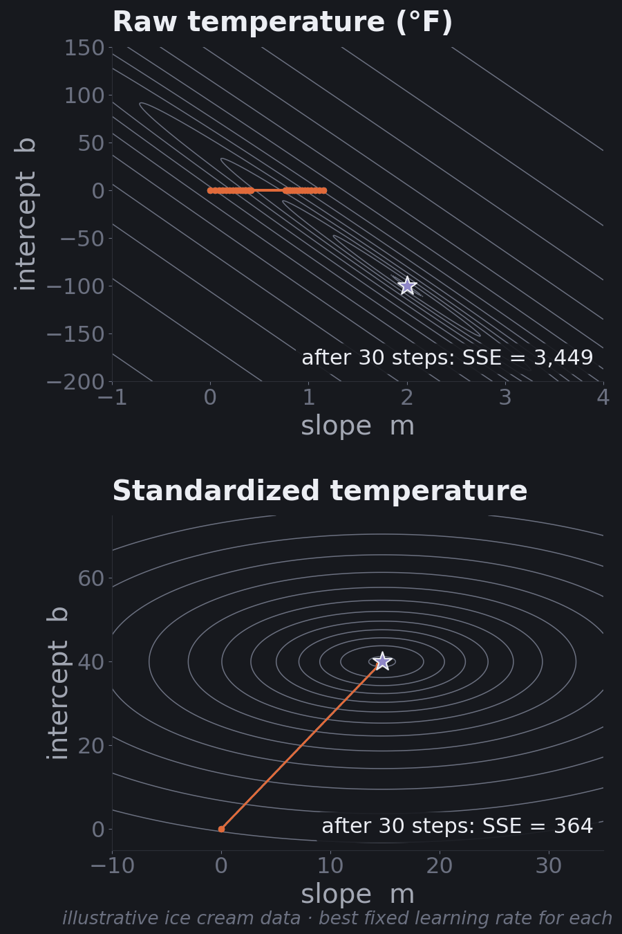
The numbers make the point. With raw temperature in °F, even the best fixed learning rate leaves the SSE at 3,449 after 30 steps, and it takes about 679,000 steps to get within 1% of the minimum. Measuring temperature from 70°F, as we have since Part 5, cuts that to 119 steps. Fully standardized, it takes 2.
The predictions don't change, only the units of the weights. That's why scaling is a standard step in any pipeline that uses gradient descent (and for distance-based models like k-nearest neighbors). One rule: compute the mean and standard deviation on the training set only, then apply them to the test set. Otherwise information about the test set leaks into training.
Part 10: The Machine Learning Workflow
Linear regression is one step in a bigger loop that every project follows:
- Define the problem. What exactly are you predicting, for whom, and how will the prediction be used? Is it classification or regression?
- Collect data. Gather examples that are relevant, representative of the cases you'll predict on, and labeled with the right answer.
- Explore and clean. Look at distributions, missing values, outliers, and errors. Plot things.
- Prepare features. Encode categories, scale numeric features, create new features where they help.
- Split. Set aside a test set before training. Fit any scaling or encoding on the training set only.
- Train. Fit the model on the training set.
- Evaluate. Compare against a simple baseline, on the test set. For regression: R², RMSE, MAE. Look at the errors, not just the summary numbers.
- Iterate. Try better features or other models, using a validation set or cross-validation, not the test set.
- Deploy and monitor. Put the model to work, and watch for its accuracy drifting as the world changes.
It's a loop, not a line. You'll bounce between steps 3 and 8 more than once. And the data steps usually matter more than the algorithm: a clean, relevant, representative dataset does more for a model than any clever technique.
The next part walks through steps 2–7 on real data.
Part 11: Hands-On: Predicting Diabetes Progression
Time to use everything on a real dataset. scikit-learn ships with the diabetes dataset from a 2004 statistics paper (Efron, Hastie, Johnstone, and Tibshirani, "Least Angle Regression"), so it needs no download. It has 442 patients. For each one, ten measurements were taken at a baseline visit: age, sex, body mass index (BMI), average blood pressure, and six blood serum measurements. The target is a number measuring how far the disease progressed one year later. Higher means worse.
The code blocks in this part (and one more in Part 12) are a single script, run top to bottom.
Load and explore
import numpy as np
import pandas as pd
from sklearn.datasets import load_diabetes

# 442 patients, 10 baseline measurements, ships with scikit-learn (no download).
# scaled=False keeps the original units (years, BMI, mm Hg, ...).
data = load_diabetes(scaled=False, as_frame=True)
df = data.frame.rename(columns={"s1": "tc", "s2": "ldl", "s3": "hdl",
                                "s4": "tch", "s5": "ltg", "s6": "glu"})
X = df.drop(columns="target")
y = df["target"]   # disease progression one year after baseline

print(X.shape)
print(X.head(3).to_string())
print(y.describe().round(1).to_string())
print(X.corrwith(y).sort_values(ascending=False).round(2).to_string())(442, 10)
age sex bmi bp tc ldl hdl tch ltg glu
0 59.0 2.0 32.1 101.0 157.0 93.2 38.0 4.0 4.8598 87.0
1 48.0 1.0 21.6 87.0 183.0 103.2 70.0 3.0 3.8918 69.0
2 72.0 2.0 30.5 93.0 156.0 93.6 41.0 4.0 4.6728 85.0
count 442.0
mean 152.1
std 77.1
min 25.0
25% 87.0
50% 140.5
75% 211.5
max 346.0
bmi 0.59
ltg 0.57
bp 0.44
tch 0.43
glu 0.38
tc 0.21
age 0.19
ldl 0.17
sex 0.04
hdl -0.39The blood measurements have short codes. The ones we'll mention: tc is total cholesterol, ldl and hdl are the "bad" and "good" cholesterol, tch is the ratio of total to HDL cholesterol, ltg is (probably, per the dataset's notes) the log of the triglyceride level, and glu is blood sugar. sex is coded 1 or 2; the dataset doesn't say which is which.
The target runs from 25 to 346 with an average of 152.1. The correlations give a first look at which single features move with it: BMI (0.59) and ltg (0.57) most strongly, then blood pressure (0.44). hdl, the "good" cholesterol, moves the other way (−0.39).
Split, baseline, fit, evaluate
from sklearn.model_selection import train_test_split
from sklearn.linear_model import LinearRegression
from sklearn.metrics import r2_score, mean_squared_error, mean_absolute_error

# Hold out 20% of patients. The model never sees them during training.
X_train, X_test, y_train, y_test = train_test_split(X, y, test_size=0.2, random_state=42)
print(f"train: {len(X_train)} patients, test: {len(X_test)} patients")

def report(name, y_true, y_pred):
    rmse = mean_squared_error(y_true, y_pred) ** 0.5
    print(f"{name:<22} R2 = {r2_score(y_true, y_pred):5.2f}   "
          f"RMSE = {rmse:5.1f}   MAE = {mean_absolute_error(y_true, y_pred):5.1f}")

# Baseline: ignore the features and always predict the training average.
baseline = np.full(len(y_test), y_train.mean())
report("baseline (test)", y_test, baseline)

model = LinearRegression().fit(X_train, y_train)
report("linear model (train)", y_train, model.predict(X_train))
report("linear model (test)", y_test, model.predict(X_test))train: 353 patients, test: 89 patients
baseline (test) R2 = -0.01 RMSE = 73.2 MAE = 64.0
linear model (train) R2 = 0.53 RMSE = 53.6 MAE = 43.5
linear model (test) R2 = 0.45 RMSE = 53.9 MAE = 42.8Line by line:
- The split. 353 patients for training, 89 held back.
random_state=42fixes which ones, so you get the same numbers. - The baseline. Ignoring every feature and predicting the training-set average (153.7) for everyone gives a test RMSE of 73.2 and MAE of 64.0. Its R² is −0.01: on new data, the training average is very slightly worse than the test set's own average, which is exactly what R² = 0 represents. Any real model has to beat this.
- The linear model on the test set: R² 0.45, RMSE 53.9, MAE 42.8. It cuts RMSE by about a quarter (73.2 to 53.9) and MAE by a third (64.0 to 42.8) compared to the baseline, and explains about 45% of the variation in progression among patients it has never seen.
- Train vs. test. R² is 0.53 on training data and 0.45 on test data. A modest gap, so not much overfitting. (The RMSEs, 53.6 vs. 53.9, are almost identical. R² dropped more because the test patients happen to vary a bit less (standard deviation 72.8 vs. 78.0 in training), so the same size of error is a bigger share of their variation. That's another reason to report error metrics alongside R².)
Is 0.45 good? It's a real improvement over guessing, and about what this dataset usually yields. But more than half the variation is unexplained, which makes sense: one year of disease progression depends on far more than ten numbers from one visit. This model could help flag higher-risk patients; it can't tell you precisely what will happen to one person.
Reading the coefficients
from sklearn.pipeline import make_pipeline
from sklearn.preprocessing import StandardScaler

# Raw coefficients: change in prediction per one unit of each feature,
# holding the other nine constant.
raw = pd.Series(model.coef_, index=X.columns)

# Standardized coefficients: same model fit on features rescaled to
# mean 0, standard deviation 1, so each is "per one standard deviation".
scaled = make_pipeline(StandardScaler(), LinearRegression()).fit(X_train, y_train)
std = pd.Series(scaled[-1].coef_, index=X.columns)

table = pd.DataFrame({"per unit": raw.round(2), "per std. dev.": std.round(1)})
print(table.reindex(std.abs().sort_values(ascending=False).index).to_string())
print(f"same predictions either way: {np.allclose(model.predict(X_test), scaled.predict(X_test))}")

# "Holding the others constant" matters: BMI's slope on its own vs. inside the full model
alone = LinearRegression().fit(X_train[["bmi"]], y_train)
print(f"bmi slope on its own: {alone.coef_[0]:.2f} inside the full model: {raw['bmi']:.2f}") per unit per std. dev.
tc -1.28 -44.4
ltg 67.11 35.2
bmi 5.85 25.6
ldl 0.81 24.6
bp 1.20 16.8
tch 10.16 13.1
sex -23.06 -11.5
hdl 0.60 7.7
glu 0.20 2.4
age 0.14 1.8
same predictions either way: True
bmi slope on its own: 10.76 inside the full model: 5.85The per unit column answers "holding the other nine features constant, how much does the predicted progression change when this feature goes up by one of its own units?"
- Each extra point of BMI adds about 5.85 to predicted progression.
- Each extra mm Hg of blood pressure adds about 1.20.
- Age adds just 0.14 per year once everything else is accounted for.
But you can't compare these to each other, because the units differ (a year of age vs. a point of BMI vs. one unit of a log scale). The per std. dev. column fixes that: same model, same predictions (the script checks), weights expressed per one standard deviation of each feature. Now BMI (25.6) and ltg (35.2) stand out as strong, consistent predictors, and age (1.8) and blood sugar (2.4) contribute little once the others are included.
The last line shows "holding others constant" at work. On its own, BMI's slope is 10.76. Inside the full model it's 5.85, because some of what BMI appeared to explain on its own is shared with blood pressure, triglycerides, and the rest.
And what about tc at −44.4, the largest weight of all, and negative, even though tc's own correlation with progression is positive (0.21)? That's not a medical finding. It's a warning sign, and Part 12 explains it.
Looking at the errors
Summary numbers hide a lot. Always plot predictions against reality and look at the residuals.
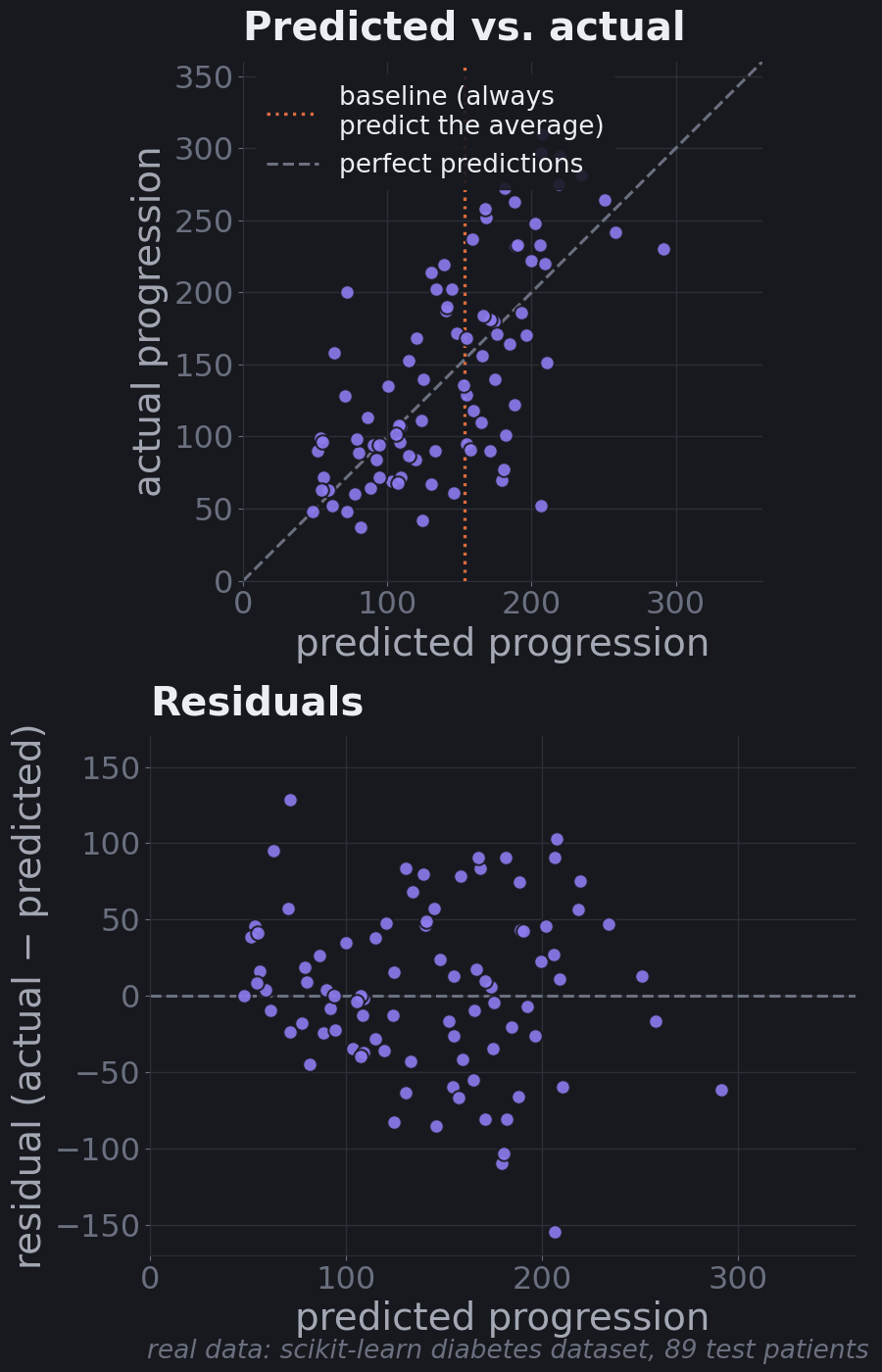
The predictions clearly track reality (the cloud runs along the diagonal), and the residuals don't show a strong curve or funnel shape, which suggests a straight-line model isn't badly wrong for this data. But individual errors of 100 or more are common. That matches the R²: useful for ranking risk, not precise for individuals.
Part 12: When Linear Regression Struggles
Linear regression makes assumptions. When they break, it still produces numbers, so you have to know what to look for.
Curved relationships
A straight line can only capture straight-line patterns. If the real relationship curves, the line will be systematically too high in some ranges and too low in others.
The best tool for spotting this is a residual plot: residuals (actual − predicted) against predictions. If the model has captured the pattern, residuals look like random noise around zero. If it has missed a curve, they form a shape.
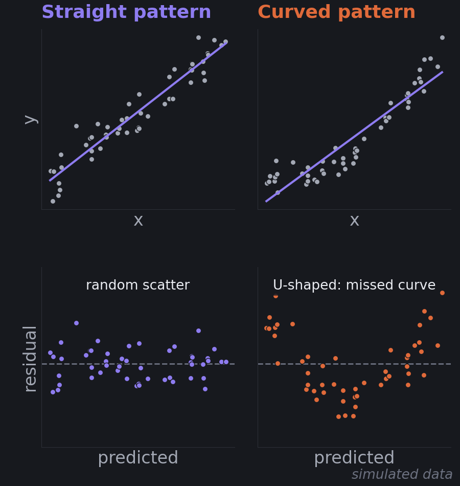
The right-hand line doesn't look terrible in the top panel, which is the point: the residual plot reveals what the fit hides. Fixes include adding curved features (like the polynomial terms from Part 8), transforming a variable (taking a logarithm is common for things like income or prices), or moving to a model that bends, like a decision tree or a neural network.
Outliers
Because errors are squared, one point far from the rest can pull the whole line toward it. A point 10 units off counts 100 times as much as a point 1 unit off.
Remember the four movies from Part 4? The $2.8B movie is far above the trend of the other three. Here's what it does to the least-squares line:
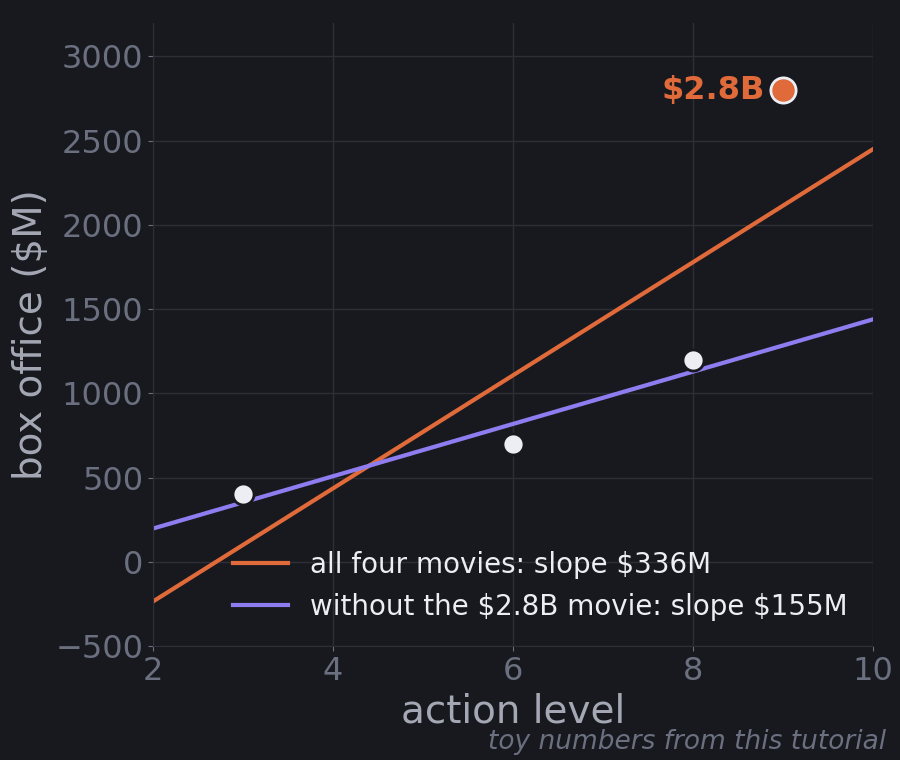
With all four movies, the best line is about −$907M + $336M × Action. Without the $2.8B movie, it's about −$113M + $155M × Action. One data point more than doubles the estimated effect of action.
What to do depends on why the point is unusual. If it's a data-entry error, fix or remove it. If it's real (blockbusters exist), don't just delete it. Consider whether your model should be predicting it at all, use a loss that squares less (MAE-style "robust" regression), or transform the target (a log scale tames big values). And always look at your data before trusting a fit.
Correlated features
When two features carry nearly the same information, the model can't tell which one deserves the credit. It can trade weight between them almost freely: a bit more on one and a bit less on the other gives nearly the same predictions. The individual weights become unstable and hard to interpret, even when the predictions are fine. This is called multicollinearity.
That's what happened with tc in Part 11. Total cholesterol includes LDL cholesterol, so the two are strongly related. Watch what happens when we drop one of them:
# tc (total cholesterol) and ldl (LDL cholesterol) measure overlapping things.
print(f"correlation between tc and ldl: {X['tc'].corr(X['ldl']):.2f}")

# Refit without one of them and compare standardized coefficients and test R2.
for dropped in [None, "ldl", "tc"]:
    cols = [c for c in X.columns if c != dropped]
    m = make_pipeline(StandardScaler(), LinearRegression()).fit(X_train[cols], y_train)
    coef = pd.Series(m[-1].coef_, index=cols)
    shown = "  ".join(f"{k} {coef[k]:+6.1f}" for k in ["tc", "ldl", "hdl", "bmi"] if k in coef)
print(f"drop {str(dropped):<5} {shown:<40} test R2 = {m.score(X_test[cols], y_test):.2f}")correlation between tc and ldl: 0.90
drop None tc -44.4 ldl +24.6 hdl +7.7 bmi +25.6 test R2 = 0.45
drop ldl tc -15.1 hdl -3.8 bmi +26.2 test R2 = 0.45
drop tc ldl -9.6 hdl -11.8 bmi +26.4 test R2 = 0.46- tc and ldl have a correlation of 0.90.
- With both in the model, tc gets −44.4 and ldl gets +24.6: large and opposite, mostly cancelling each other out.
- Drop ldl and tc shrinks to −15.1. hdl even flips sign, from +7.7 to −3.8.
- Drop tc instead and ldl flips from +24.6 to −9.6.
- Test R² barely moves (0.45, 0.45, 0.46), and BMI stays steady around 26 throughout.
So the predictions were never the problem. The interpretation was. If you'd reported "total cholesterol strongly reduces disease progression" from the first model, you'd have been reading noise. Before interpreting weights, check how your features correlate. Fixes include dropping or combining redundant features, or using regularization (ridge regression in particular spreads weight more evenly across correlated features).
Part 13: Where This Leads
From a line to a probability: logistic regression
Linear regression predicts numbers. What about classification, like Family Friendly or not?
You might try fitting a line to labels coded 0 and 1. It sort of works, but the line happily predicts −0.3 or 1.4, which make no sense as probabilities. The fix is to keep the linear score and squash it through an S-shaped curve called the sigmoid:
$$p = \sigma(w \cdot x + b) = \frac{1}{1 + e^{-(w \cdot x + b)}}$$
The inside, \(w \cdot x + b\), is exactly the linear mapping from Part 4. The sigmoid turns any score into a number between 0 and 1. Very negative scores go to nearly 0, very positive scores to nearly 1, and a score of 0 gives exactly 0.5.
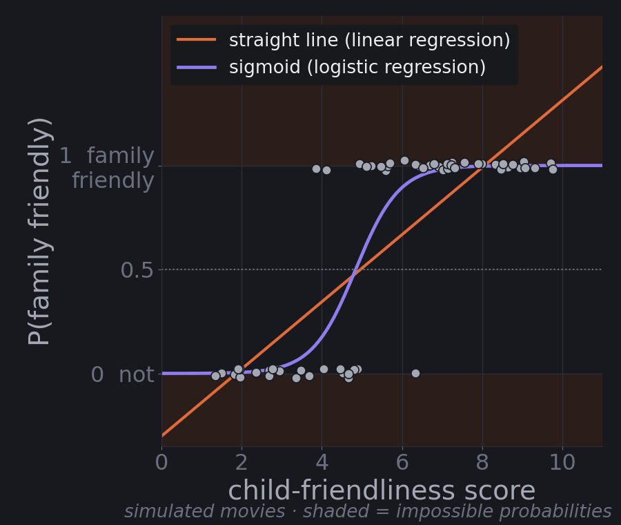
That's logistic regression, despite the name a classification model. The point where the probability crosses 0.5 is the decision boundary, the "invisible line between neighborhoods" from Part 3. Training works the same way you've seen: define an error (for probabilities, a measure called log loss rather than squared error), then walk downhill with gradient descent. The next tutorial, Classification Models, starts there and adds k-nearest neighbors, decision trees, and Naive Bayes.
Same picture, different shapes
Every model you'll meet next fits the same geometric picture. They differ in what shape they find in feature space and how they measure error:
| Model | What it finds in feature space | How it learns |
|---|---|---|
| Linear regression | A flat mapping (line, plane, hyperplane) to a number | Minimize squared error |
| Logistic regression | A flat boundary between classes | Minimize log loss |
| Decision trees | Boxes, by splitting one feature at a time | Choose splits that make each box as pure as possible |
| Support vector machines | The boundary with the widest possible gap between classes | Maximize that margin, penalizing violations |
| k-nearest neighbors | No explicit shape; it looks up the closest training points | Nothing to fit; it stores the data |
| Neural networks | Many linear mappings stacked, with bends in between | Minimize error with gradient descent, at scale |
So when you meet a new algorithm, ask three questions: What shape is it finding in feature space? How does it measure its errors? How does it minimize them? You now have the vocabulary to answer all three.
Key Takeaways
- Machine learning finds rules from examples instead of following hand-written rules. Supervised learning learns from examples with the right answer attached.
- Data is geometry. Every object becomes a vector, a point in feature space. Classification draws boundaries between regions; regression maps points to a number.
- Linear regression learns a mapping: weights that turn a feature vector into a prediction through a dot product. Each weight is the effect of one feature holding the others constant.
- Find the pattern, make predictions, minimize errors. The best line minimizes the sum of squared errors, and gradient descent finds it by stepping downhill on the error bowl. The learning rate sets the step size, and feature scaling makes the bowl round enough to walk down quickly.
- Explained vs. unexplained. \(R^2\) measures the explained share of the variation; RMSE and MAE measure the size of the errors in real units. Always compare to a baseline.
- Generalization is the real score. Evaluate on a held-out test set. Too simple underfits; too flexible overfits, with low training error and high test error.
- Know the failure modes: curves (check residual plots), outliers (squared error amplifies them), and correlated features (unstable, misleading weights).
- The same ideas carry forward. Wrap the linear score in a sigmoid and you have logistic regression. Stack many mappings with bends between them and you have a neural network.
Next: Classification Models · Also see: Neural Networks Demystified
Comments (0)