Neural Networks Demystified: Transformations Through Embedding Spaces
Neural networks can seem like mysterious "black boxes." You feed in data, numbers get multiplied somewhere inside, and a prediction comes out. But there is a simple, intuitive way to understand what is happening inside:
A neural network is a series of pattern detectors, arranged in layers. Each layer looks at the data, asks "which of my patterns are present here, and how strongly?", and passes the answers on as a new list of numbers. Layer by layer, raw data is turned into a representation where the final prediction becomes easy.
The goal of training, then, is to learn the weights and biases that make the right detectors switch on for the right inputs. A well-trained network:
- switches on a detector when its pattern is present in the input,
- keeps it switched off when the pattern is absent,
- and through those on/off decisions, places similar inputs close together and pushes different inputs apart.
This article builds that picture one step at a time, using a single running example: predicting house prices. We'll go through:
- How data becomes a list of numbers, and why that list can be treated as a point in space
- What a layer of neurons is, what it produces, and how big it should be
- What a single neuron computes, and why it acts as a pattern detector
- What the activation function (ReLU) does, and why a network can't work without it
- A complete walk-through of houses passing through a small network
- What stacking layers lets a network learn that a simple formula can't, including the classic XOR problem and how the same ideas work on images
- How neurons come to detect different patterns
- How the final layer makes a prediction, how training tunes everything, and what can go wrong
We'll finish with answers to a few common questions.
We'll keep the math light. Every formula in this article is a multiplication, an addition, or "keep the number if it's positive, otherwise use zero." The goal is a clear mental model of what each part of a network is doing and why.
Step 1: Data as Points in Space
A neural network only works with numbers. Before any learning can happen, every input has to be turned into a vector: a list of numbers that describes the item.
How that happens depends on the kind of data:
- Images: a small 28×28 grayscale image has 784 pixels. Each pixel's brightness becomes one number, so the image becomes a list of 784 numbers.
- Words: a word like "king" can be turned into a list of, say, 300 numbers using a method like Word2Vec or GloVe, or a learned embedding layer inside the network. The numbers are learned so that words used in similar ways get similar lists.
- Tables: each row is one item and each column is one feature. A row with columns for age, income, and education level becomes a vector of three numbers.
- Categories: a value like "city" or "product type" is usually mapped to a short learned vector through an embedding lookup table: one row of numbers per category. This is more compact than one-hot encoding, which would need a separate 0/1 column for every possible category.
Vectors Are Points
Here is the idea that the rest of this article builds on: a vector can be thought of as a point in space, with one dimension per number.
- A table row with three columns is a point in 3-dimensional space. You could plot it on three axes: age, income, education.
- A 784-pixel image is a point in 784-dimensional space. We can't picture 784 axes, but the math works exactly the same way as with three.
- A 300-number word vector is a point in 300-dimensional space.
We call such a space an embedding space, and an item's point in it is its embedding.
Similar Items Sit Close Together
Why think of data as points? Because distance becomes meaning. Items that share similar features have similar numbers, so their points land near each other:
- Images of the same handwritten digit have many pixels in common, so they cluster together.
- Words with similar meanings, like "queen" and "prince," land near "king."
- People with similar ages, incomes, and education levels sit near each other in a table's space.
So where a point sits tells you what the item is like, and the direction from one point to another tells you how two items differ.
Directions can carry meaning too. In a good word embedding, the step from "man" to "woman" points in roughly the same direction as the step from "king" to "queen." That's why the famous arithmetic works approximately: start at "king," subtract "man," add "woman," and the nearest word is "queen." The space has organized itself so that a direction means something like "make it female." (The Word2Vec article shows how those embeddings are learned.) Keep this idea in mind: in Step 3 we'll see that a neuron is, in a sense, a detector for one particular direction.
As we'll see, everything a neural network does can be described as moving points around: taking the points from one space and placing them in a new space where the things that matter for the task are easier to see.
Our Running Example: House Prices
Throughout this article, we'll predict house prices from three features:
- x₁: house size (square feet)
- x₂: number of bedrooms
- x₃: age of the house (years)
Here is a small dataset:
| House | Size (sq ft) | Bedrooms | Age (years) | Price ($K) |
|---|---|---|---|---|
| 1 | 2500 | 4 | 2 | 1300.8 |
| 2 | 1800 | 3 | 25 | 945.9 |
| 3 | 1200 | 2 | 5 | 649.6 |
| 4 | 3500 | 5 | 40 | 1793.5 |
| 5 | 800 | 1 | 1 | 450.1 |
Each house becomes a vector of its three features:
- House 1:
[2500, 4, 2] - House 2:
[1800, 3, 25] - House 3:
[1200, 2, 5] - House 4:
[3500, 5, 40] - House 5:
[800, 1, 1]
These vectors are the network's inputs. The prices are the targets: the answers the network should learn to produce. The network's job is to take a vector like [1800, 3, 25] and predict a price as close as possible to 945.9.
Why Features Are Scaled First
There is one practical problem with these raw numbers. Compare House 1 and House 2. Their sizes differ by 700 square feet, their bedrooms by 1, and their ages by 23 years. If we measure the distance between their points, we get about 700.38. If we ignore age completely, the distance is 700.0007. The 23-year age difference barely registers, simply because square footage is measured in bigger numbers.
The same thing happens inside a network: a feature with big numbers drowns out features with small numbers, no matter which one actually matters more. So before training, features are usually scaled to similar ranges. A common choice is to rescale each feature so that 0 means "average for this dataset," positive means "above average," and negative means "below average." Whenever we compare features in the examples below, we'll use scaled values like these.
Step 2: Layers of Neurons
A neural network is built from layers, and data flows through them in order:
- The input layer receives the vector, such as
[1800, 3, 25]. It doesn't compute anything; it just holds the numbers. - The hidden layers sit in between. This is where the learning happens.
- The output layer produces the final prediction, such as
945.9.
A hidden layer is called "hidden" because its values never appear in the data or in the output. They are the network's internal working: its own description of the input.
Each Neuron Answers One Question
A hidden layer is made of neurons (also called nodes or units). Each neuron looks at the whole input vector and produces one number. You can think of each neuron as asking one question about the input, such as "is this a big, new house?", and the number it outputs is its answer: how strongly it sees its pattern.
A layer has many neurons, each asking a different question. So if a layer has three neurons, it produces three numbers for every house. Those three numbers form a brand-new vector.
Each Layer Builds a New Embedding Space
This is the central idea of the article. The new vector is a point in a new embedding space, but the axes of this new space mean something different. In the input space, the axes were "size," "bedrooms," and "age." In the new space, the axes are "how much of pattern 1 is present," "how much of pattern 2," and "how much of pattern 3."
So a layer doesn't just pass the data along. It re-describes every input in terms of the patterns it has learned to look for, and in doing so, it moves every point to a new place. Inputs that trigger similar patterns land close together in the new space, even if their raw numbers looked quite different. Inputs that trigger different patterns are pushed apart.
The next layer then does the same thing again, starting from the new space. Each layer builds a new, more useful view of the data, tailored to the task, whether that's predicting house prices, recognizing handwritten digits, or translating a sentence.
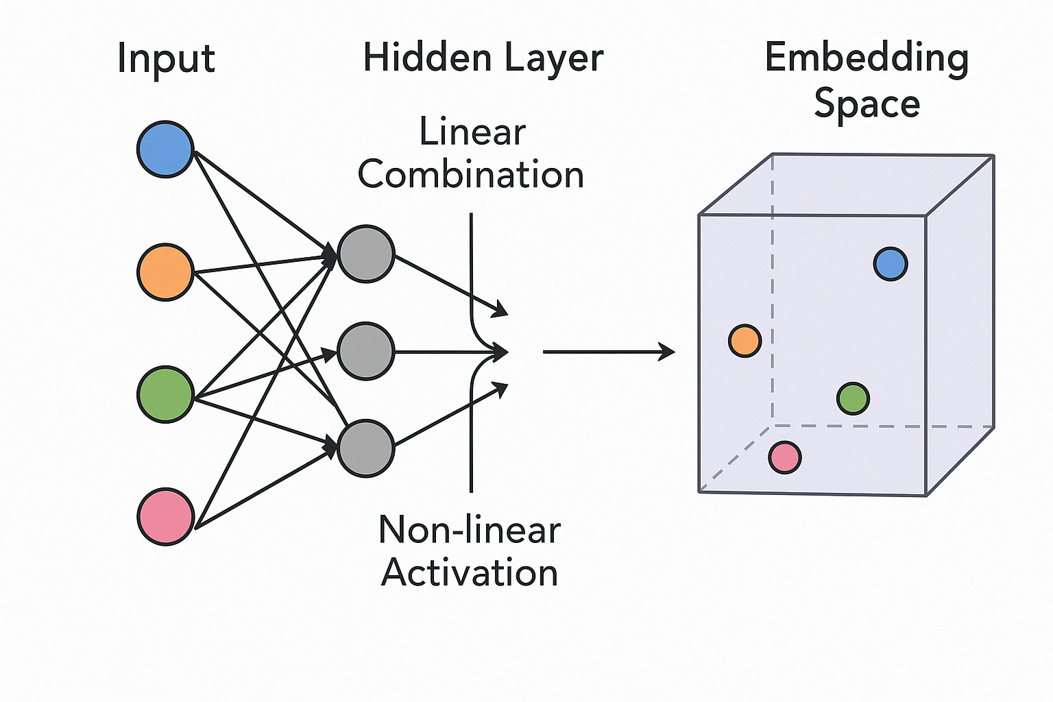
The image shows this for houses. On the left, each house is described by its features: size, bedrooms, and age. These are combined into a vector and passed into the hidden layer. Inside the hidden layer, each neuron computes how strongly it sees its pattern in that house.
If the hidden layer has three neurons, every house comes out as a new vector of three numbers. One house might become [2.0, 0.0, 1.5]: strong on pattern 1, completely absent on pattern 2, fairly strong on pattern 3.
On the right side of the image, each house is drawn as a point in this new space. Houses with similar characteristics land closer together, and houses that differ are placed farther apart. That organization is what makes the final prediction easier: once similar houses sit together, predicting a price is a matter of knowing which region of the space a house falls in.
Weights and Biases: What a Layer Learns
In a fully connected (or "dense") layer, every neuron is connected to every input. To decide how much each input matters, a neuron has:
- one weight for each input feature, and
- one extra number called a bias.
Think of each input feature as a separate piece of information about the house. A neuron's job is to combine all of those pieces into one answer, so it needs to decide how much attention to pay to each piece. That's what the weights are: one "how much does this feature matter to me" number per feature. If the input has 3 features, every neuron in the first hidden layer needs exactly 3 weights. (We'll see what the bias does in Step 3.)
So with I input features and N neurons, a layer has:
$$ \text{parameters} = (I \times N) + N $$
The \(I \times N\) part counts the weights, and the \(+N\) adds one bias per neuron. For example, with our 3 house features and a hidden layer of 4 neurons:
- each neuron has 3 weights and 1 bias, for 4 parameters,
- so the layer has \(4 \times 4 = 16\) parameters.
These parameters are the only things a network learns. Everything a trained network "knows" is stored in its weights and biases.
How Many Neurons Should a Layer Have?
The number of weights per neuron is fixed by the data: one per input feature. But the number of neurons in a layer is a design choice. Since each neuron is a pattern detector, the number of neurons is the number of patterns the layer can look for.
- With too few neurons, the layer may not have enough detectors to capture the patterns that matter.
- With too many neurons, the network has so much freedom that it can memorize the training examples, including their noise, instead of learning patterns that carry over to new data.
There is no formula for the right number. The usual approach is to start small, try a few sizes, and keep the one that performs best on validation data: examples held back from training to check how well the network generalizes.
Wider or Deeper?
There are two ways to give a network more capacity: add more neurons to a layer (making it wider), or add more layers (making it deeper). They do different things.
- A wider layer has more detectors looking at the same input. It can recognize more patterns side by side, but each pattern is still built directly from that layer's inputs.
- A deeper network lets later layers build patterns out of earlier layers' patterns. A neuron in layer 3 can detect "a combination of combinations," something no single layer can express on its own.
In practice, depth is usually the more efficient way to add power. Many real-world patterns are naturally layered (strokes make shapes, shapes make digits; features make conditions, conditions make concepts), and a deep network can mirror that structure with far fewer neurons than one very wide layer would need. That's where the "deep" in deep learning comes from. We'll see why layering is so powerful in Step 6.
Step 3: Inside a Neuron
Now let's open up a single neuron and see what it computes. It does three simple things with the input vector:
- multiplies each input by its weight,
- adds the results together,
- adds its bias.
$$ z = w_1x_1 + w_2x_2 + \cdots + w_nx_n + b $$
This is called a weighted sum or linear combination, and the result is a single number, \(z\). The whole input vector, however many numbers it has, is collapsed into one number.
What That Number Means
Here is the key to understanding neural networks. A neuron is a pattern detector. Its weights describe the pattern it is looking for, and \(z\) measures how strongly the current input matches that pattern:
- High \(z\): a strong match. The pattern is clearly present.
- \(z\) near zero: the input has little to do with the pattern.
- Negative \(z\): the input is the opposite of the pattern.
Notice what a neuron does not decide: whether its pattern actually matters for predicting the price. That is learned during training, through how much the next layer listens to this neuron. A neuron simply reports what it sees.
An Example
Take a neuron that looks at two house features, size and age, both scaled so that 0 means "average." Its weights are [1, −1]:
$$ z = (1 \times \text{size}) + (-1 \times \text{age}) $$
Being bigger pushes \(z\) up, and being older pushes it down. So the pattern this neuron detects is "big and new." If you drew the weights as an arrow on a plot of size vs. age, it would point right (bigger) and down (newer): the neuron is a detector for that direction, and \(z\) measures how far a house goes that way. Here are four houses:
| House | Size | Age | z = size − age |
|---|---|---|---|
| A: big, new | 1.5 | −1.0 | 2.5 |
| B: big, old | 1.5 | 1.2 | 0.3 |
| C: small, new | −1.0 | −1.0 | 0 |
| D: small, old | −1.0 | 1.5 | −2.5 |
House A fits the pattern completely, so it scores highest. House D is the exact opposite, so it scores lowest. Houses B and C each match only half the pattern, so their two features cancel out and they land near zero.
How Weights Shape the Pattern
Each weight has two jobs:
- Its sign decides which way a feature pushes. A positive weight on size means "bigger counts in favor." A negative weight on age means "older counts against."
- Its size decides how much the feature counts. If the size weight were 2 instead of 1, size would count twice as much as age. A weight of 0 means the neuron ignores that feature entirely.
By choosing different weights, a neuron can describe any pattern built from its inputs. Weights of [1, 0] make a pure "big house" detector that ignores age. Weights of [0, 1] make an "old house" detector. Weights of [2, −1] make a detector for "big and new, but mostly big." Training is the process of finding the weights that describe useful patterns.
One thing to keep in mind: \(z\) also grows with the size of the input. A house that is extremely big and extremely new will score even higher than house A. So a large \(z\) means "this input has a lot of the pattern," which is one more reason features are scaled to similar ranges before training: we want the score to reflect the pattern, not just which feature happens to be measured in big numbers.
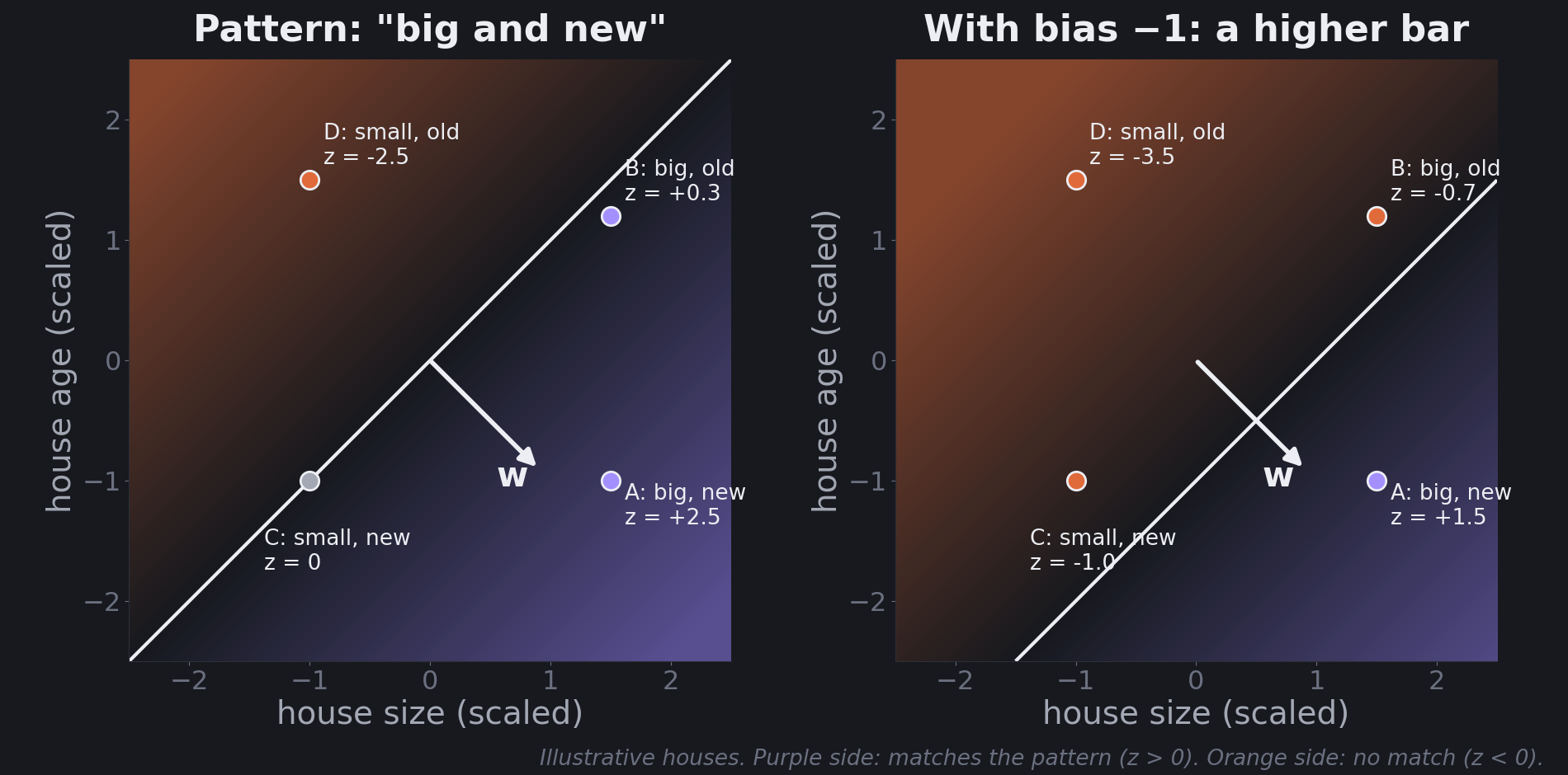
The Bias Sets the Bar
The last ingredient is the bias. The bias adds the same amount to every score, no matter what the input is. That makes it a threshold: it controls how strong a match has to be before the neuron's score turns positive.
- A negative bias raises the bar. The input needs a stronger match to get a positive score.
- A positive bias lowers the bar. Even a weak match gets a positive score.
In the right panel of the figure, the "big and new" neuron gets a bias of −1:
$$ z = \text{size} - \text{age} - 1 $$
Now a house needs size − age to be greater than 1 before \(z\) turns positive. House A still passes easily (2.5 − 1 = 1.5). But house B, which scored 0.3 before, drops to −0.7. Being big is no longer enough to make up for being old: B doesn't count as a "big and new" house anymore.
Without a bias, the dividing line between "match" and "no match" would always sit at exactly zero, which here means an average house. The bias lets each neuron put its line wherever it is most useful. One neuron might fire only for houses that are much bigger than average; another might fire for anything above average. The same weights with different biases give detectors that are pickier or more lenient about the same pattern.
So the three parts of a neuron's score divide the work neatly:
- the weights say what to look for,
- the bias says how strong the match must be,
- and \(z\) is the result: how strongly this input matches, after the bar is applied.
Step 4: The Activation Function (ReLU)
After computing \(z\), the neuron passes it through an activation function, which decides what the neuron actually sends to the next layer. The most widely used one is ReLU (Rectified Linear Unit):
$$ \text{ReLU}(z) = \max(0, z) $$
That's all it does: keep positive scores as they are, and turn negative scores into zero. In pattern-detector terms:
- Pattern present (\(z > 0\)): the neuron "fires" and passes on how strong the match is.
- Pattern absent (\(z \le 0\)): the neuron outputs exactly zero. It stays silent for this input.
Here is the "big and new" neuron (with no bias) after ReLU:
| House | z | ReLU(z) |
|---|---|---|
| A: big, new | 2.5 | 2.5 |
| B: big, old | 0.3 | 0.3 |
| C: small, new | 0 | 0 |
| D: small, old | −2.5 | 0 |
House D's −2.5 has become 0. The neuron doesn't say "this house is very much not big and new." It simply says nothing. Only houses that have the pattern get a signal through.
Silence Is the Point
This might look like throwing information away, but it is exactly what makes a neuron a true detector rather than just a weighted average. For any given house, only the neurons whose patterns are present contribute to the next layer. The rest are switched off.
And crucially, a different house switches on a different set of neurons. A big new house might activate one group of detectors, and a small old house a completely different group. Each house's new vector records which patterns it has and how strongly, and nothing else. Many of the numbers are exactly zero, which is why these vectors are called sparse.
That gives the next layer a clean signal. Instead of sorting through every detector's opinion about every input, it receives only the patterns that are actually present. A zero isn't permanent, though: it only applies to this one input. The same neuron that is silent for house D fires strongly for house A.
Other Activation Functions
ReLU isn't the only option. Sigmoid squashes any score into the range 0 to 1, and tanh squashes it into −1 to 1. Both were common in early networks, and sigmoid is still used at the output when a network must produce a probability. But inside hidden layers, ReLU and its close variants are the usual choice: they are cheap to compute, and they make deep networks much easier to train. The ideas in this article hold for any of them: what matters is that the function is non-linear, meaning it isn't just "multiply by a number and add a number."
Why We Can't Skip It
What if we dropped the activation function and let every neuron pass its score straight through? Two things go wrong.
First, depth stops mattering. A layer without an activation function just multiplies and adds. And multiplying and adding twice is still just multiplying and adding. Take a one-number example. Suppose layer 1 computes \(z_1 = 2x + 1\), and layer 2 computes \(z_2 = 3z_1 - 4\). Put them together:
$$ z_2 = 3(2x + 1) - 4 = 6x - 1 $$
The two layers are identical to a single layer with weight 6 and bias −1. The same thing happens with any number of inputs and neurons: stacking 3, 10, or 100 layers without activation functions gives you exactly what one layer could give you. The whole network collapses into a single weighted sum, which is just linear regression.
Second, nothing can be switched on or off. Without ReLU, every neuron passes something forward for every input, so every pattern always affects the result, whether it's present or not. A linear model can learn to ignore a feature everywhere by giving it a weight of zero. What it can't do is use a feature for some houses and ignore it for others. Every feature pushes the price by the same amount, for every house.
The next two steps show what we gain by keeping the activation function: first in a complete example, then in the kinds of patterns it makes possible.
Step 5: One House, All the Way Through
Let's put everything together and follow houses through a complete (tiny) network. To keep the numbers readable, we'll use our four houses with just two scaled features, size and age, and we'll pick the weights by hand so each neuron's job is easy to see. A trained network finds its own weights, but it does exactly this arithmetic.
The Network
The hidden layer has three ReLU neurons, each a detector for one pattern:
| Neuron | Weights (size, age) | Bias | Computes | Detects |
|---|---|---|---|---|
| h₁ | [1, −1] | 0 | ReLU(size − age) | "big and new" |
| h₂ | [0, 1] | −1 | ReLU(age − 1) | "clearly old" |
| h₃ | [−1, 0] | 0 | ReLU(−size) | "small" |
The output neuron combines their answers into a price (in thousands of dollars):
$$ \text{Price} = 1000 + 200\,h_1 - 150\,h_2 - 250\,h_3 $$
Read it like a pricing rule: start at \$1,000K, add value for "big and new," and take value away for "clearly old" and for "small."
The Forward Pass
House A (big, new): size 1.5, age −1.0
- h₁ = ReLU(1.5 − (−1.0)) = ReLU(2.5) = 2.5
- h₂ = ReLU(−1.0 − 1) = ReLU(−2.0) = 0
- h₃ = ReLU(−1.5) = 0
New vector: [2.5, 0, 0]. Price = 1000 + 200 × 2.5 = \$1,500K.
House B (big, old): size 1.5, age 1.2
- h₁ = ReLU(1.5 − 1.2) = 0.3
- h₂ = ReLU(1.2 − 1) = 0.2
- h₃ = ReLU(−1.5) = 0
New vector: [0.3, 0.2, 0]. Price = 1000 + 200 × 0.3 − 150 × 0.2 = 1000 + 60 − 30 = \$1,030K.
House C (small, new): size −1.0, age −1.0
- h₁ = ReLU(−1.0 − (−1.0)) = 0
- h₂ = ReLU(−1.0 − 1) = 0
- h₃ = ReLU(1.0) = 1.0
New vector: [0, 0, 1.0]. Price = 1000 − 250 × 1.0 = \$750K.
House D (small, old): size −1.0, age 1.5
- h₁ = ReLU(−1.0 − 1.5) = ReLU(−2.5) = 0
- h₂ = ReLU(1.5 − 1) = 0.5
- h₃ = ReLU(1.0) = 1.0
New vector: [0, 0.5, 1.0]. Price = 1000 − 150 × 0.5 − 250 × 1.0 = 1000 − 75 − 250 = \$675K.
What Just Happened
Look at the new vectors side by side:
| House | Input (size, age) | Hidden vector (h₁, h₂, h₃) | Price |
|---|---|---|---|
| A: big, new | (1.5, −1.0) | [2.5, 0, 0] | \$1,500K |
| B: big, old | (1.5, 1.2) | [0.3, 0.2, 0] | \$1,030K |
| C: small, new | (−1.0, −1.0) | [0, 0, 1.0] | \$750K |
| D: small, old | (−1.0, 1.5) | [0, 0.5, 1.0] | \$675K |
Everything from the earlier steps is visible here:
- Each neuron answered one question. h₁ answered "how big and new?", h₂ "how clearly old?", h₃ "how small?"
- ReLU kept each answer honest. Every neuron that didn't see its pattern output exactly 0. Most entries in the hidden vectors are zeros.
- Each house switched on different neurons. A lit up only the "big and new" detector. C lit up only the "small" detector. D lit up "small" and "clearly old."
- The hidden layer moved the houses to a new space. C and D, the two small houses, now sit close together ([0, 0, 1.0] and [0, 0.5, 1.0]), because they share the pattern that matters most for them. A sits far from both, alone on the "big and new" axis.
- The output layer only had to read off the patterns. Once the houses were described by their patterns, pricing them was a simple weighted sum.
Try Changing One Number
To feel how the parts fit, change a single parameter and rerun the houses. Suppose we change h₂'s bias from −1 to 0, so it computes ReLU(age) instead of ReLU(age − 1). We've lowered the bar: h₂ is no longer a detector for "clearly old," just for "older than average."
- House A (age −1.0): h₂ = ReLU(−1.0) = 0. Nothing changes: still \$1,500K.
- House C (age −1.0): h₂ = 0 again. Still \$750K.
- House B (age 1.2): h₂ = ReLU(1.2) = 1.2, so the penalty grows from 30 to 150 × 1.2 = 180. Price = 1000 + 60 − 180 = \$880K (was \$1,030K).
- House D (age 1.5): h₂ = 1.5, so the penalty grows from 75 to 225. Price = 1000 − 225 − 250 = \$525K (was \$675K).
One bias changed, and only the houses with that pattern were affected. The new houses didn't move at all, because the detector stayed silent for them. That is the kind of targeted adjustment a linear model can't make, and it is exactly the kind of adjustment training makes, thousands of times over.
That is the whole story of a neural network, in miniature. Bigger networks have more inputs, more neurons, and more layers, and their weights are learned rather than chosen by hand, but every neuron in them does exactly what h₁, h₂, and h₃ just did.
Step 6: What Non-Linearity Makes Possible
We've seen that ReLU lets neurons switch on and off. Now let's see why that matters so much, by looking at what a model without it can't do.
What a Linear Model Can Do
A model with no activation functions is a linear model: the output is a weighted sum of the inputs plus a bias, just like a single neuron. For our five houses, this linear formula fits every price exactly:
$$ \text{Price} = 500x_1 + 300x_2 - 200x_3 + 50000 $$
Reading it term by term:
- each square foot adds \$500,
- each bedroom adds \$300,
- each year of age subtracts \$200,
- and the bias, \$50,000, is the starting value before any features are counted.
(A bedroom is worth surprisingly little here because size already captures most of what extra bedrooms bring: bigger houses tend to have more bedrooms, so once the model knows the size, the bedroom count adds little new information.)
The Assumptions Built Into It
That formula is easy to read, but it bakes in three strong assumptions:
- Each feature always has the same effect. The model says each bedroom adds \$300, so going from 1 to 2 bedrooms adds \$300, and going from 5 to 6 also adds \$300. In reality, buyers might value the second bedroom far more than the sixth.
- Features don't interact. The value of one feature never depends on another. A pool would add the same amount to every house, whether it's in Phoenix or in Alaska. An extra bedroom would add the same amount to a tiny house as to a mansion.
- Boundaries are straight lines. Suppose houses are "expensive" only when they are over 2,000 square feet and under 20 years old. On a plot of size vs. age, the "expensive" region is a corner: everything to the right of the 2,000 line and below the 20-year line. A linear model can't draw a corner. It can only draw one straight line across the plot, so some houses near the corner will always land on the wrong side.
Real data breaks these assumptions all the time. Values level off, effects depend on context, and categories have irregular shapes. Here is how ReLU neurons handle each of these, using only the tools we already have: weights, a bias, and ReLU.
1. Thresholds
Say houses start losing value quickly once they pass 30 years old. Below that, age barely matters. A linear model can only say "each year costs the same amount." But one ReLU neuron can detect exactly this situation.
Give the neuron a weight of 1 on age, 0 on size and bedrooms, and a bias of −30:
$$ a = \text{ReLU}(0 \cdot x_1 + 0 \cdot x_2 + 1 \cdot x_3 - 30) = \text{ReLU}(\text{age} - 30) $$
- A 25-year-old house gives ReLU(−5) = 0. The neuron stays silent.
- A 35-year-old house gives ReLU(5) = 5. The neuron fires, and its output says how far past 30 the house is.
This is the bias at work as a threshold: the weights picked the feature (age), and the bias of −30 put the bar at 30 years. The neuron is a detector for "older than 30," and the next layer can attach a steep price drop to it, a drop that only applies to houses that have crossed the line. A linear model could reduce the importance of age, but it could never ignore age below 30 and use it above 30.
2. Effects That Change Over the Range
Now suppose bedrooms have diminishing returns: the first bedroom adds \$50,000, the second adds \$30,000, and every bedroom after that adds only \$10,000. A linear model can't do this, because its bedroom weight is the same for every bedroom. Three ReLU neurons can:
| Neuron | Computes | Turns on at | Output weight |
|---|---|---|---|
| A | ReLU(bedrooms) | 1st bedroom | +\$50,000 |
| B | ReLU(bedrooms − 1) | 2nd bedroom | −\$20,000 |
| C | ReLU(bedrooms − 2) | 3rd bedroom | −\$20,000 |
Here is how they work together:
- Neuron A counts every bedroom, and its weight adds \$50,000 per bedroom.
- Neuron B only starts counting at the second bedroom (thanks to its bias of −1). Its weight subtracts \$20,000 per bedroom from then on, so each bedroom from the second onward is worth \$50,000 − \$20,000 = \$30,000.
- Neuron C only starts counting at the third bedroom. It subtracts another \$20,000, so each bedroom from the third onward is worth \$30,000 − \$20,000 = \$10,000.
Check it:
- 1 bedroom: A = 1 → \$50,000. B and C are silent. Total \$50,000.
- 2 bedrooms: A = 2 → \$100,000; B = 1 → −\$20,000; C is silent. Total \$80,000: the second bedroom added \$30,000.
- 4 bedrooms: A = 4 → \$200,000; B = 3 → −\$60,000; C = 2 → −\$40,000. Total \$100,000: the third and fourth bedrooms added \$10,000 each.
Notice the trick. Each neuron doesn't add a fixed amount; it bends the line at its threshold, changing the slope from that point on. Add up enough of these bends and a network can follow almost any curve, built out of short straight pieces. This is one of the most important facts about neural networks: with enough ReLU neurons, they can approximate essentially any smooth relationship between inputs and output.
3. Combinations of Features
The third limitation, features that interact, is where stacking layers comes in. Each layer can detect patterns made of the previous layer's patterns. Suppose our inputs include the number of bedrooms, the climate, the size, and whether the house has a pool.
Layer 1: simple conditions. Each neuron detects one basic condition, using a weight and a bias as a threshold:
- one neuron fires when there are more than 3 bedrooms,
- one fires when the house is in a hot climate,
- one fires when the house is over 2,000 square feet,
- one fires when there is a pool.
The output of this layer is a new vector where each number means "this condition is present, this strongly." That is already a more useful description than the raw features.
Layer 2: combinations. The neurons in this layer see Layer 1's outputs as their inputs. So a Layer 2 neuron can give positive weights to two Layer 1 neurons and use its bias to set the bar high enough that both must be firing for it to turn on:
- one neuron fires only when "over 2,000 sq ft" and "has a pool" are both active,
- another fires only when "hot climate" and "more than 3 bedrooms" are both active.
This layer's vector describes the house in terms like "large house with a pool" or "family-size home in a hot region."
Layer 3: higher-level concepts. Neurons here combine the combinations. One might fire only when "large house with a pool" and "hot climate" are both active. It can then learn a rule like:
"A pool adds a lot of value, but only for large houses in hot climates."
That is a conditional rule: the value of one feature (the pool) depends on others (size and climate). A linear model could never express it, because it gives the pool one fixed value everywhere. And none of these conditions were columns in the data. The network built them, one layer at a time, out of nothing but weighted sums, biases, and ReLU.
The Classic Test: XOR
There is a famous small problem that shows the limits of linear models in the cleanest possible way. It's called XOR, short for "exclusive or." Take two yes/no features, each either 0 or 1. The answer should be 1 when exactly one of them is 1, and 0 otherwise:
| Feature 1 | Feature 2 | XOR |
|---|---|---|
| 0 | 0 | 0 |
| 1 | 0 | 1 |
| 0 | 1 | 1 |
| 1 | 1 | 0 |
Plot the four cases as points on a square. The two "1" answers sit on opposite corners, and the two "0" answers sit on the other two corners. No single straight line can put both 1s on one side and both 0s on the other. Try it: any line that separates one 1 from the 0s puts the other 1 on the wrong side. So no linear model, and no single neuron, can solve XOR. In 1969, Marvin Minsky and Seymour Papert pointed out this limit of single-layer networks, and it cooled interest in neural networks for years.
Two ReLU neurons and an output solve it easily. Let \(s\) be the sum of the two features, and compute:
- h₁ = ReLU(s): "at least one feature is on," and how many,
- h₂ = ReLU(s − 1): "both features are on" (the bias of −1 sets the bar at two),
- output = h₁ − 2h₂.
Check all four cases:
- (0, 0): s = 0, so h₁ = 0 and h₂ = 0. Output 0.
- (1, 0): s = 1, so h₁ = 1 and h₂ = 0. Output 1.
- (0, 1): s = 1, so h₁ = 1 and h₂ = 0. Output 1.
- (1, 1): s = 2, so h₁ = 2 and h₂ = 1. Output 2 − 2 = 0.
The second neuron is a detector for "both," and the output uses it to cancel the case the first neuron gets wrong. This is the same trick as the bedroom example: a second ReLU, switching on at a higher threshold, bends the result. In a house-price model, the same structure lets a network learn things like "either a home office or a guest room adds value, but having both doesn't add twice as much."
4. Specialists for Different Situations
Because a ReLU neuron stays silent unless its pattern is present, groups of neurons can end up acting like specialists, each handling a different kind of house:
- Young homes: neurons computing something like ReLU(20 − age) fire only for houses under 20 years old. A 15-year-old house gives 5; a 25-year-old house gives 0. These neurons can learn what matters for newer homes, such as modern layouts or energy efficiency.
- Very old homes: neurons computing ReLU(age − 50) fire only for houses over 50 years old. A 60-year-old house gives 10; a 45-year-old house gives 0. These neurons can learn about renovation costs or historic value.
- Luxury in hot climates: a deeper neuron that fires only when both "has a pool" and "hot climate" are active, learning that a pool adds more value where it's used year-round.
Each group stays silent unless its situation comes up. So in effect, the network contains several small models inside it, and for each house, only the relevant ones speak. That is a big part of how one network can handle very different kinds of inputs.
Why Deep Networks Work
Put all of this together, and each layer re-describes the input in terms of more useful patterns than the layer before:
- Early layers detect simple patterns: thresholds, the presence or absence of a feature. In image models, these are edges, corners, and textures.
- Middle layers combine simple patterns into interactions. In images, these are shapes and parts: an eye, a wheel, a letter stroke.
- Later layers capture high-level concepts that make the prediction easy. In images, these are whole objects: a face, a car, a digit.
The same layering appears in other kinds of data. Language models develop detectors that respond to grammatical structures, topics, or tone. Audio models develop detectors for frequencies, pitch patterns, and speech sounds. None of these patterns are programmed in. Nobody tells a neuron "look for edges" or "look for pools in hot climates." They emerge from training, because they help reduce the prediction error.
The Same Idea in Images
Houses make the arithmetic easy to follow, but the pattern-detector idea is easiest to see in images. Take a network that reads 28×28 handwritten digits, so each input is 784 pixel brightnesses.
A neuron in the first hidden layer has 784 weights, one per pixel. Here's the neat part: you can arrange those 784 weights back into a 28×28 grid and look at them as a picture. The picture is the neuron's pattern.
Suppose a neuron's weights look like this:
- positive along a vertical strip down the middle,
- negative in the areas on either side of it,
- near zero everywhere else.
Now feed it an image. Each bright pixel is multiplied by the weight at the same position, and everything is added up:
- If the digit has a vertical stroke down the middle, its bright pixels land on the positive weights. \(z\) is high. This neuron is a vertical-stroke detector, and it fires.
- If the digit's ink lands mostly on the negative areas, beside the strip, \(z\) goes negative, and ReLU silences the neuron.
- If the image is mostly blank where the weights are, \(z\) stays near zero.
The bias plays its usual role: it decides how much stroke is enough. A strongly negative bias means the neuron only fires for a long, clear stroke; a smaller one lets a short or faint stroke through.
So the first layer is a bank of templates: strokes at different angles and positions, curves, blobs. When researchers draw the first-layer weights of a trained digit network as images, they do often see stroke-like shapes, though usually noisier and less tidy than a human would draw them.
The second layer then works with the first layer's answers, not with pixels. One of its neurons might give positive weights to "curve at the top," "curve at the bottom," and "closed loop," and fire for an 8. Another might combine "vertical stroke" with "short horizontal stroke near the top" to fire for a 7. Each layer asks its questions in terms of the previous layer's patterns, exactly like the bedrooms-climate-pool example, just with pixels instead of house features.
Step 7: How Neurons Come to Specialize
That raises a natural question. If nobody tells each neuron which pattern to detect, why don't they all end up detecting the same thing? In practice, different neurons do end up specializing, for a few reasons:
- Different starting points. Every neuron starts with its own random weights, so from the very first step each one is slightly tuned to something different. Training amplifies those small differences.
- Learning dynamics. When a neuron is slightly better than the others at responding to some pattern, it gets the strongest updates for that pattern during training. That makes it better still, and it gradually "claims" the pattern.
- Training rewards new information. Two neurons that detect exactly the same pattern add little that one couldn't. Nothing in training explicitly forbids this, but the fastest way to reduce the overall error is usually for neurons to cover different parts of the problem, so the gradients tend to reward a neuron for capturing something the others missed.
An Example From Handwritten Digits
In a network trained to recognize handwritten digits, you might find:
- one neuron that responds to loops, like those in 0, 6, 8, and 9,
- another that responds to vertical strokes, like those in 1, 4, and 7,
- a third that responds to diagonal strokes, like those in 2 and 7.
No one programmed these roles. They emerged because they are useful for telling digits apart.
Why Some Overlap Remains
Specialization is rarely perfect, and some overlap is actually helpful:
- Partial sharing. Several neurons may detect versions of the same pattern that differ slightly in angle, position, or scale.
- Distributed representations. Important patterns are usually captured by a group of neurons working together rather than by one neuron alone.
- Robustness. If one neuron fails to fire on an unusual input, another with an overlapping pattern may still respond.
Engineers sometimes encourage specialization with sparsity constraints, which limit how many neurons can be active at once, or with competitive mechanisms, where neurons compete for the right to respond to a pattern. Dropout, which randomly switches neurons off during training, is sometimes mentioned in the same breath, but it pushes the other way: it stops neurons from relying on each other, so useful patterns end up spread across more neurons. That makes the network more robust, which is why dropout is so widely used.
Step 8: The Output Layer and Training
The Final Prediction
After the last hidden layer, the data reaches the output layer. For predicting a house price, this is usually a single neuron with no ReLU, because a price can be any number and we don't want negative scores clipped to zero. It takes the last hidden layer's vector \(h_1, \ldots, h_n\) and computes one more weighted sum:
$$ \text{Price} = w_1h_1 + w_2h_2 + \cdots + w_nh_n + b $$
This is exactly what the output neuron in Step 5 did with [h₁, h₂, h₃]. Each weight says how much one pattern is worth in dollars. A positive weight means the pattern raises the price; a negative weight means it lowers it. The bias is the starting price before any patterns are counted.
For example, a house with 2,500 square feet, 4 bedrooms, and 2 years of age might reach the last hidden layer as a vector like [3.2, 0.0, 5.1]: strong on two patterns, silent on one. The output neuron weighs those pattern strengths and turns them into a price.
The output layer also handles scale. The hidden layers deal in pattern strengths like 0.3 or 2.5, but our prices range from about \$450,000 to \$1.8 million. The output layer's weights and bias stretch and shift the result into the right range. Nobody sets this by hand: training adjusts those weights until the predictions land in the same range as the real prices.
Other Kinds of Output
House prices are a regression task: the answer is a number. For other tasks, only the output layer changes. The hidden layers, the pattern detectors, work exactly the same way.
- Yes/no questions ("will this house sell within 30 days?"): the output neuron's weighted sum goes through a sigmoid, which squashes it into a probability between 0 and 1.
- Choosing among several classes ("which digit is this?"): there is one output neuron per class, ten for digits, and a function called softmax turns their scores into probabilities that add up to 1. Each output neuron is, once again, a pattern detector: its pattern is "the hidden-layer patterns that add up to a 7."
The loss function changes with the task too. Mean squared error suits prices, because it measures how far off a number is, and it punishes big misses much more than small ones. For probabilities, networks use cross-entropy, which punishes confident wrong answers most heavily. Either way, it plays the same role in training: one number that says how wrong the network was.
Similar Inputs, Similar Predictions
Because similar houses trigger similar patterns, they reach the output layer as similar vectors, and the same weights turn similar vectors into similar prices. We saw this in Step 5: the two small houses, C and D, ended up with nearby vectors and nearby prices.
This is also why a network can price a house it has never seen. A new house is run through the same detectors, lands near the training houses it resembles, and gets a price like theirs. Nobody wrote a rule saying "group similar houses together." The structure emerges from training, because grouping similar houses is the easiest way to predict their prices accurately.
How Training Tunes Everything
In Step 5, we picked the weights by hand. A real network starts with random weights and biases, so at first its "patterns" are meaningless and its predictions are poor. Training fixes this by repeating a simple loop:
- Forward pass. Run a house through the network, exactly as in Step 5, to get a predicted price.
- Loss. Compare the prediction to the real price using a loss function, such as mean squared error, which turns "how wrong was that?" into a single number.
- Backpropagation. Work backward through the network to figure out how much each weight and bias contributed to the error. This uses calculus (the chain rule), but the idea is simply assigning blame.
- Gradient descent. Nudge every weight and bias a little in the direction that reduces the error.
One Nudge, Step by Step
Let's see one round of this on house B from Step 5. Our network predicted \$1,030K. Suppose the real price is \$1,100K. The prediction is \$70K too low.
The output neuron's three weights were 200, −150, and −250, and house B's hidden vector was [0.3, 0.2, 0]. Training asks, for each weight: if I change this weight, how much does the prediction move? The answer is just the neuron output it multiplies:
- The "big and new" weight (200) multiplies h₁ = 0.3. Raising it raises the prediction, which is what we want. With a small learning rate (0.1, using squared error), it moves up to 204.2.
- The "clearly old" weight (−150) multiplies h₂ = 0.2. Making it less negative raises the prediction, so it moves to −147.2.
- The "small" weight (−250) multiplies h₃ = 0. Changing it wouldn't affect this prediction at all, so it stays at −250.
- The bias (1000) affects every prediction directly, so it moves up to 1014.
With the new values, house B's prediction becomes 1014 + 204.2 × 0.3 − 147.2 × 0.2 = \$1,045.8K. The error shrank from \$70K to about \$54K in a single step.
Notice the third bullet. A neuron that was silent for this house gets no blame and no update. The "small" detector had nothing to do with house B's prediction, so training leaves it alone. This is ReLU's on/off behavior showing up again, this time in learning: each example only adjusts the detectors that were involved in it.
The same idea flows backward through the hidden layer: backpropagation also works out how h₁'s and h₂'s own weights and biases should change, so the detectors themselves gradually shift toward more useful patterns.
Many Passes Over Many Houses
One nudge only fixes one house a little. Training repeats the loop over every house in the dataset, and then over the whole dataset again and again. Each full pass is called an epoch. The nudges from different houses pull in slightly different directions, and over many epochs they settle on weights that work well for all of them.
By the end, the hidden neurons have become useful pattern detectors, the output layer knows what each pattern is worth, and the network predicts well, not only on the training houses, but on new houses it has never seen. That ability to generalize is the real goal of training.
What Can Go Wrong
The training loop is simple, but a few things commonly go wrong, and each one makes sense in terms of the pattern-detector picture.
Memorizing instead of learning (overfitting). Our table has 5 houses, and even a small hidden layer of 4 neurons on 3 features has 16 parameters before we count the output layer. A network with more adjustable numbers than examples can simply memorize every price, using its detectors to recognize individual houses rather than general patterns like "big and new." It will look perfect on the training data and fail on new houses. The fixes are more data, smaller networks, and always checking performance on held-out validation data that the network never trains on. Real house-price models train on thousands of sales, not five.
Steps that are too big or too small. The learning rate controls how far each nudge goes. Too small, and training crawls. Too large, and each nudge overshoots: the weights jump past the good values, the error grows instead of shrinking, and training can blow up entirely. The Introduction to Machine Learning tutorial shows this happening with real numbers.
Detectors that never fire ("dead" neurons). We saw that a silent neuron gets no update. That's usually good, but it has a failure mode: if a neuron's weights and bias end up so that \(z\) is negative for every input, it never fires, so it never gets blamed, so it never changes. It is stuck off for good. This "dying ReLU" problem is why careful weight initialization and moderate learning rates matter, and why variants like Leaky ReLU exist: instead of outputting exactly zero for negative scores, Leaky ReLU lets a tiny fraction through (for example, 0.01 × z), so a silent neuron still gets a small update and can recover.
Unscaled features. We met this in Step 1. If size is in thousands and bedrooms are in single digits, the size weights dominate every score at the start, and gradient descent takes a long, zig-zagging path to good weights. Scaling features first is one of the cheapest and most effective things you can do.
Common Questions
Is a neuron like a brain cell? Only loosely. The name comes from a rough analogy: a biological neuron collects signals from other cells and "fires" when the total is strong enough, which is a bit like a weighted sum followed by ReLU. But an artificial neuron is just a small math function, and a neural network doesn't work the way a brain does. The analogy is useful for intuition, not as a description of biology.
Do real neurons detect clean, human-readable patterns like "big and new"? Sometimes, but often not. In our examples, we chose weights by hand so every neuron had one tidy job. In a trained network, some neurons do respond to recognizable patterns, like strokes in images. But many respond to mixtures of several patterns, and many useful patterns are spread across groups of neurons rather than living in one. Working out what trained networks have learned is an active research area called interpretability. The pattern-detector picture is still the right mental model; the patterns just aren't always ones we have names for.
Why do neural networks need so much data? Because they have so many parameters, and each one is learned from examples. Every weight is shaped by many small nudges, each from one example. With too few examples, there isn't enough evidence to tell real patterns apart from coincidences, and the network ends up memorizing (see "What Can Go Wrong" above). Simple models with a handful of parameters, like the linear formula in Step 6, can get by with far less data, which is one reason they are still widely used.
Why not always use a neural network instead of linear regression? When the relationship really is close to linear, or when data is limited, a linear model is often just as accurate, much easier to interpret, and much harder to overfit. Neural networks earn their extra complexity when the data has thresholds, curves, and interactions, and when there is enough data to learn them reliably.
Conclusion
Neural networks look complicated, but they are built from one simple idea, repeated many times: a neuron is a pattern detector.
- Data becomes points in space. Every input is turned into a vector, and similar inputs sit close together.
- Each neuron computes a weighted sum. Its weights describe a pattern, and its score says how strongly the input matches.
- The bias sets the bar for how strong a match must be.
- ReLU lets a neuron fire only when its pattern is present. That on/off behavior is what lets a network handle thresholds, curves, combinations of features, and different kinds of inputs.
- Each layer builds a new embedding space, re-describing every input in terms of the patterns it contains, so that similar inputs end up together and the final prediction becomes easy.
- The output layer turns pattern strengths into a prediction, and training tunes every weight and bias, one small nudge at a time, until the patterns are the useful ones.
We kept the math light here on purpose. The natural next step is the mechanics behind training: how gradient descent uses derivatives, how the learning rate controls the size of each step, and how the chain rule carries the blame backward through many layers. The Introduction to Machine Learning tutorial works through gradient descent and the learning rate in code on a simple linear model, and the RNN tutorial shows backpropagation at work in a small network written from scratch.
Comments (0)